Investigations on the finite strain behavior of standard PVB: experiment and modeling

Source: Glass Structures & Engineering

Authors: Alexander Pauli & Geralt Siebert

DOI: https://doi.org/10.1007/s40940-024-00247-2

Abstract

The numerical simulation of the residual load-bearing capacity of laminated glass is one of the most relevant topics of current research in structural glass engineering. The mechanical description of the behavior of the interlayer plays a crucial role. Several approaches and models already exist in automotive engineering and structural protection. Structural glass design assuming quasi-static loads misses a detailed model so far. The aim of this work is the mechanical description of the time-dependent behavior of Polyvinylbutyral (PVB) under large deformations considering quasi-static loading. The results of experiments on single-layer Standard PVB are presented, and a model of finite nonlinear viscoelasticity is derived. In particular, the formulation of phenomenologically motivated viscosity functions is described. Subsequently, the model parameters are calibrated on the experimental results, and the uniaxial stress state is simulated.

1 Introduction

Nowadays, glass is one of the most widely used materials for structures with high requirements for aesthetics and transparency. It applies to facades, pedestrian bridges, canopies, and fall-protecting balustrades. In most applications, there are increased requirements for the residual load-bearing capacity and minimizing the risk of injury in the event of breakage. The use of laminated safety glass is mandatory in this respect, and the assessment of the residual load-bearing capacity is an integral part of the design process. The numerical description of the residual load-bearing capacity is part of current research in structural glass design. The modeling of the material behavior of the interlayer, which undergoes large deformations in the fractured state, plays a decisive role. This work investigates the time-dependent behavior of PVB under large deformations experimentally, describes it mechanically, and simulates it numerically. Guided by the normative requirements for the experimental determination of the residual load-bearing capacity, the investigations are limited to one specific temperature and relative humidity.

The work consists of six parts. (1) the content of the paper is introduced, and a brief outline of the current state of research on PVB at large strains and modeling finite viscoelasticity, in general, is given; (2) the material is described, and the mechanical background is settled; (3) the experimental investigations are introduced and the results are presented; (4) the material model is constructed, respective parameters are calibrated and the tests are simulated (5) the quality of the model is evaluated and discussed (6) the work is summarized, and further research needs are outlined.

In recent years, many experimental studies have been conducted on PVB. Hooper et al. (2011); Kuntsche (2015); Xu et al. (2016); Pelfrene (2016); Knight et al. (2022); Pauli and Siebert (2023) investigated the behavior of PVB at finite strains under quasi-static loading. Kuntsche (2015); Kraus and Niederwald (2017); Kraus et al. (2018); Kraus (2019); Schuster (2023), explored the time-dependent behavior at small deformations assuming linear viscoelastic material behavior. Elzière (2016) explored the loading and unloading behavior of PVB at large strains and different temperatures besides the linear viscoelastic behavior at small strains. Furthermore, Schuster et al. (2021) investigated the limits of the application of the theory of linear viscoelasticity to modeling PVB. Botz et al. (2019) investigated the influence of humidity. In conclusion, PVB shows a strongly nonlinear behavior at large strains, along with a time, temperature and humidity dependency.

There are several modeling approaches for PVB at large strains for the application in structural glass design. Kuntsche (2015); Kraus (2019); Pauli and Siebert (2023) used hyperelastic material models. Pelfrene (2016); Alter et al. (2017) described the behavior using linear viscoelastic, large deformation models. However, to the author’s knowledge, there is no model for PVB accounting for large deformation nonlinear viscoelasticity yet.

1.1 General frameworks for finite viscoelasticity and -plasticity

The following sections describe models that already exist in the literature. Two kinds are distinguished: models that describe the behavior of elastomers and models that describe the behavior of thermoplastics. The basic framework is the same for both types. It follows the structure of a single Maxwell element, comprised of spring and damper. However, the formulation of the dashpot decides whether the material model is viscoelastic or viscoplastic. The material behavior is viscoplastic if it depends on a set of equations containing yield criterion and flow rule with rate dependency and viscoelastic if the formulation only depends on a rate-dependent flow rule without any yield criterion.

However, in both cases, a multiplicative split of the deformation gradient into elastic and inelastic components must be carried out to apply these concepts to large deformations. The multiplicative split goes back to Lee (1969), who derived it for plasticity, and Lubliner (1985), who transferred it to viscoelasticity. The structure of the Maxwell element can be enriched by a parallel spring, yielding the three-parameter Maxwell element. The material response of the single spring is referred to as equilibrium stiffness, as it represents the state of thermomechanical equilibrium by an elastic curve. A parallel friction element can be added to this equilibrium response, leading to a rate-independent equilibrium hysteresis. The response of the Maxwell element is referred to as non-equilibrium stiffness, as it represents the distance away from the thermomechanical equilibrium. 

Further, single Maxwell or other rheological elements can supplement these simple models. However, within large deformations, it is common practice that all elastic responses, referred to as springs, are based on hyperelastic energy potentials. The flow rules incorporated in the dashpots depend on respective viscosities. Amongst others, there are two common approaches. Reese and Govindjee (1998) used a dissipation potential to derive the flow rule. This potential is a scalar-valued, non-negative function that depends on all thermodynamic forces and potentially corresponding process variables and must adhere to the requirements of convexity. On the other hand, Lion (2000) suggested the description of the relationship between the inelastic deformation rate and the associated stresses in terms of general tensor functions of the thermomechanical process history. An excellent overview of the possible formulations of viscosity functions is given by Lion (2000).

1.2 Models for elastomers

Reese and Govindjee (1998) and Middendorf (2001) provided basic frameworks for the modeling and FE implementation of finite viscoelastic materials. Reese and Govindjee (1998) used a formulation accounting for compressible behavior, Middendorf (2001) used a formulation based on incompressibility. The framework proposed by Middendorf (2001) was extended to thermo-viscoelasticity by Heimes (2004).

Bergström and Boyce (1998) created a viscoplastic model for carbon-filled rubber based on the rheological structure of the three-parameter Maxwell model. Their approach is micromechanically motivated and divides the model into different networks describing different kinds of polymer chains and their intrinsic connections. The flow rule includes reptational motion and contour length variations, considering Brownian movements within a constrained tube. The potential for the elastic and the inelastic material response is derived from the 8-chain model of Arruda and Boyce (1993).

Lion (1996) developed a viscoplastic model for rubber containing carbon black, with an underlying assumption of incompressibility. Within this model, equilibrium and non-equilibrium responses are derived from potentials of the Mooney-Rivlin type (Mooney 1940; Rivlin 1948). Notably, this model incorporates a damage parameter, accounting for the Mullins effect, and a relaxation time contingent upon the total stress history.

Sedlan and Haupt (1999) adopted a modeling approach for viscoelastic materials based on the framework provided by Lion (1996). In their model, the viscosity function is intricately linked to an internal variable that captures the influence of thixotropy and two additional process variables that account for the rate and magnitude of deformation. For the equilibrium component of their model, they extended the Mooney-Rivlin model. The non-equilibrium responses of the material are described using Neo-Hookean potentials (Treloar 1943).

Koprowski-Theiß (2011) proposed a viscoelastic model designed to capture the intricate behavior of nonlinear finite viscoelasticity in porous rubber containing carbon black. Within this model, the equilibrium component is established based on the potential formulation introduced by Yeoh (1990). The non-equilibrium behavior is described by a series of modified Neo-Hookean elements . Its evolution equation is influenced by process-dependent relaxation times. They are contingent upon the extent of deformation and the deformation rates experienced by the material.

By introducing additional non-equilibrium elements, Scheffer (2016) expanded upon the framework established by Koprowski-Theiß (2011). In doing so, Scheffer augmented the Neo-Hookean elements with a modified Yeoh potential and a distinct formulation of the viscosity functions. Additionally, Scheffer’s model operates under the assumption of incompressible material behavior.

Justine (2008) described the behavior of mineral nonwovens for a wide temperature range, considering isothermal processes. She decomposed the viscoelastic model into isochoric and volumetric parts, using the compressible formulation of Blatz and Ko (1962). Furthermore, the flow rule incorporates a temperature-dependent viscosity and a structure variable accounting for thixotropic effects.

Schröder et al. (2021) investigated self-heating phenomena of elastomers and therefore expanded the classical generalized viscoelastic Maxwell model by a thermocouple in series. The underlying potentials in their model adhere to the Neo-Hookean potential formulation. The model’s evolution equation incorporates a temperature-dependent constant and follows the Williams-Landel-Ferry (WLF) formulation (Williams et al. 1955).

1.3 Models for thermoplastics

Boyce et al. (1988) developed a viscoplastic constitutive model describing the behavior of glassy polymers at large deformations. This model is based on the macromolecular description of the material, incorporating micromechanical effects, following the rheological structure of a single Maxwell element with a spring in parallel. The initial response, representing the intermolecular resistance, is governed by the tensor of elasticity that acts on the natural logarithm of the elastic deformation gradient (Anand 1979) and a term accounting for temperature effects. The damper of the Maxwell element follows a plastic flow rule based on the double kink model of Argon et al. (1985) and accounts for rate and temperature dependency. The network resistance is modeled by entropic hardening using the model of Wang and Guth (1952) based on non-Gaussian statistics to describe the respective back stress tensor.

This model was expanded by Boyce et al. (2000) who developed a constitutive model for poly(ethylene terephthalate) (PET) at temperatures above the glass transition temperature using a parallel network of two Maxwell elements A and B. Network A describes the initial stiffness represented by intermolecular interactions. The formulation of Anand (1979) describes its elastic response; the inelastic response is similar to that of Boyce et al. (1988). Network B describes the molecular resistance of the material. The hyperelastic model proposed by Arruda and Boyce (1993) governs its elastic response; its inelastic response follows a similar expression to the one proposed by Bergström and Boyce (1998). However, it additionally considers strain-induced crystallization.

Dupaix and Boyce (2007) developed a model describing the experimental investigations on the finite strain behavior of poly(ethylene terephthalate) (PET) and poly(ethylene terephthalate)-glycol (PETG) discovered by Dupaix and Boyce (2005). The model follows the concept presented by Boyce et al. (2000). However, they use a strongly temperature-dependent shear modulus for the initial stiffness of the elastic spring of network A.

Mulliken and Boyce (2006) modeled polycarbonate and poly(methyl methacrylate) at high strain rates or low temperatures. They expanded the two-network model by a parallel spring following the description of Arruda and Boyce (1993) describing the network resistance. The intermolecular resistance is decomposed into two rate-activated processes presented by the two Maxwell elements. The first part considers rotations of the polymer main-chain segments, and the second considers intermolecular resistance.

A model for Polyetheretherketone (PEEK) and (PC), following the same principle structure, was recently proposed by Zhu et al. (2021).

1.4 Outline

Although PVB shows nonlinear viscoelastic material behavior within the regime of large deformations Kuntsche (2015); Schuster (2023), the modeling approaches reach from linear viscoelastic (Kuntsche 2015; Kraus and Niederwald 2017; Kraus et al. 2018; Kraus 2019; Schuster 2023) over hyperelastic (Kuntsche 2015; Kraus 2019; Pauli and Siebert 2023) to finite linear viscoelastic descriptions (Pelfrene 2016; Alter et al. 2017). These approaches cannot accurately describe the complex behavior of PVB within the regime of large deformations. However, in polymer mechanics, several models exist that are qualitatively capable of describing such behavior (Reese and Govindjee 1998; Sedlan and Haupt 1999; Justine 2008; Koprowski-Theiß 2011; Scheffer 2016). This work aims to adopt a general framework of finite viscoelasticity (Middendorf 2001) to describe the time-dependent material behavior of PVB utilizing a combination of several Maxwell elements comprised of respective hyperelastic potentials and nonlinear viscosity functions.

2 Methodology

In this section, the focus is on presenting an in-depth examination of the materials under investigation and establishing the mechanical principles, essential for modeling the material behavior. For a comprehensive understanding, the section is structured into the three distinct components, “Material,” “Mechanical Background,” and “Finite Viscoelasticity”.

2.1 Material

PVB takes center stage in this study as it’s a widely utilized material for interlayers in laminated glass applications.

It is predominantly composed of three key elements: PVB resin, constituting approximately 75% of the material, additives (less than <1%), and plasticizer, which makes up around 25%. Notably, the proportion of plasticizers plays a pivotal role in determining the material’s glass transition temperature. The higher the plasticizer content, the lower the glass transition temperature. Kraus (2019); Schuster (2023)

The synthesis of PVB involves a sequence of chemical processes. It commences with the chain polymerization of vinyl acetate, followed by hydrolysis to produce polyvinyl alcohol. Subsequently, acetalization with butyraldehyde occurs, leading to the formation of PVB. A crucial feature of PVB is its amorphous thermoplastic nature, characterized by a lack of crosslinks. Additionally, it exhibits purely viscoelastic and isotropic behavior. Kraus (2019); Schuster (2023)

The specific PVB material employed in this study is provided by Kuraray Europe GmbH and marketed as TrosifolUltraClear - B200NR. It possesses a glass transition temperature of approximately 25∘C and a Poisson’s ratio of approximately 0.47, as reported in previous studies. (Kuntsche 2015; Kraus 2019)

2.2 Mechanical background

The theories of small and large deformation viscoelasticity both share a common rheological foundation, exemplified by the three-parameter Maxwell model. This foundation is built on the fundamental concept of separating the Green-Lagrange strain tensor into its elastic and inelastic components. The flow rule of viscoelasticity determines the distribution of elastic and inelastic deformation. The split of the Green-Lagrange strain tensor plays a crucial role in this concept. For small deformations, this split can be carried out in an additive manner. However, when dealing with large deformations, further considerations are necessary to adapt and apply this concept.

This study demonstrates the transition from modeling linear, small deformation viscoelasticity to modeling nonlinear, large deformation viscoelasticity. Therefore, we will elucidate the fundamental kinematics and establish the modeling framework. Starting at the displacement of a particle, which is defined as follows:

From this formulation, the deformation gradient can be derived as follows:

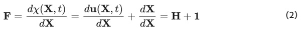
where H equals the displacement gradient. The expression of the Green-Lagrange strain tensor leads to:

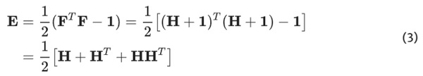
In the context of small deformations, it is possible to linearize the Green-Lagrange strain tensor by omitting the term HHᵀ, which is small of higher order. As a result, the linearized strain tensor is expressed as follows:

It can be split into an elastic eₑₗ and inelastic component eᵢₙ, in analogy to the single Maxwell element.

In the case of large deformations, the additive split described earlier is no longer possible because the nonlinear term HHᵀ cannot be omitted. The deformation gradient must be multiplicatively divided into an elastic Fₑₗ and an inelastic part Fᵢₙ to establish an additive split following the Maxwell model:

The concept of a multiplicative split, introduced by Lee (1969) for plasticity and later applied to viscoelasticity by Lubliner (1985), involves a fictitious intermediate configuration. Haupt and Tsakmakis (1989) provided a comprehensive concept and the corresponding transformation rules to establish this theory within a thermodynamically consistent framework. For additional material modeling concepts and related references, readers are encouraged to consult sources such as (Haupt 2000; Holzapfel 2002; Simo and Hughes 2006). Applying the concept proposed by Haupt and Tsakmakis (1989) results in the description of the deformation tensor of the inelastic intermediate configuration (Γ^):

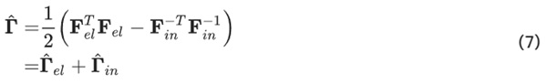
where

equals the elastic part (of the Green type) and

equals the inelastic part (of the Almansi type). These deformations can be conceptualized as the deformation of spring and damper within a single Maxwell element, akin to the scenario of small deformations. The magnitudes of elastic and inelastic deformation are governed by a particular flow rule.

2.3 Finite viscoelasticity

The proposed model builts up on the work of Middendorf (2001) and is based on the Clausius Duhem inequality considering isentropic and isothermal processes. Formulated on the reference configuration, it yields:

where T equals the Second Piola Kirchhoff stress tensor (2ⁿᵈPK) operating on the reference configuration, ρ₀ equals the density (in the following considered within the potentials), Ψ equals the Helmholtz Free Energy, and ()˙=d/dt equals the derivative with respect to time.

It is common practice to split up the energy Ψ into a part describing the thermodynamical equilibrium Ψ∞(E) and a part describing the distance away from the thermodynamical equilibrium Ψ^ᵒᵛ(Γ^ₑₗ). The equilibrium potential depends on the reference configuration. However, following the concept of Dual Variables (Haupt and Tsakmakis 1989), the non-equilibrium potential depends on the inelastic stretch tensor that operates on a stress-free intermediate configuration (Bergström and Boyce 1998). To ensure physical consistency Eq. 8 must be transformed to the intermediate configuration for establishing the flow rule and then transformed back to the reference configuration to obtain the Total Lagrangian formulation. The total stress with respect to the reference configuration results in:

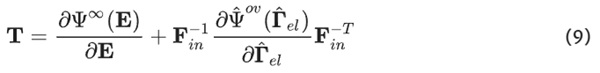
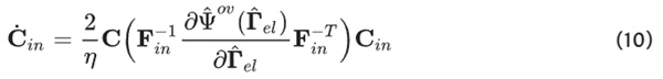
With the introduction of the proportionality factor η, referred to as viscosity, to satisfy the dissipation inequality, the viscoelastic flow rule results in:

Since Ψ^ᵒᵛ(Γ^ₑₗ) and Ψ∞(E) are isotropic tensor functions, they can be expressed in terms of the invariants of the right Cauchy-Green stretch tensor C and its elastic part

which is the counterpart to the inelastic part of the stretch tensor

This goes along with the formulation of the potentials depending on invariants. To account for nearly incompressible material behavior these potentials can be divided into deviatoric and volumetric parts. This split also applies to Eq. 9 and Eq. 10, while for Eq. 10 the relation proposed by Justine (2008) is used. Along with the temperature dependency of PVB, the underlying deformation gradient is partitioned into a mechanical segment FM and a thermal counterpart Fθ to account for isothermal processes at different temperatures (Lion 2000):

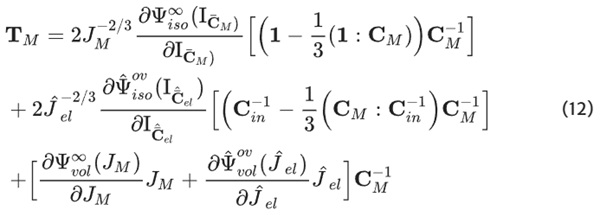
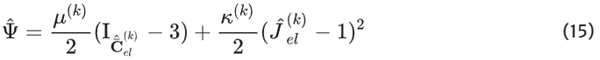
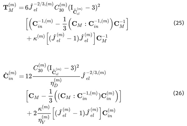
The thermal component is computed in advance, guided by a priori considerations, while the mechanical part is subsequently substituted. The final expression of the finite viscoelastic material model accounting for isothermal processes based on energy potentials that depend only on the first invariant, results in the following total stress:

and the flow rule:

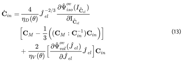
While for Eq. 13 the relations ηᵥ=αηD and α>0 must hold for volumetric (ηᵥ) and deviatoric (ηD) viscosities (justine 2008). Furthermore, 

equalis the mechanical right Cauchy-Green stretch tensor, J and J^ₑₗ the determinats of the deformation gradient and its elastic part, IC¯M and IC¯^ₑₗ, the first invariant of the right Cauchy-Green stretch tensor and its elastic part, and θ the temperature.

3 Experiments

In this chapter, the results of the experimental investigations are presented, and we commence with a detailed account of the conditioning and preparation of the test specimens. Following this, we provide a comprehensive overview of the fundamental experimental procedure.

Our attention then turns to the presentation of various test specifications, each selected due to its direct relevance to the numerical calculation of the residual load-bearing capacity of laminated safety glass. Within this context, we scrutinize three pivotal phenomena:

1. Rate-dependent Behavior: The stress response under varying strain rates is investigated.
2. Hysteresis Behavior: The examination of hysteresis behavior reveals the energy dissipation characteristics of laminated safety glass.
3. Relaxation Behavior: A crucial aspect of our investigation is to analyze the material’s capacity to relax from fixed deformation over time.

These investigations are pivotal in our quest to understand the mechanical performance of laminated safety glass, contributing essential insights that form the basis of our numerical calculations for residual load-bearing capacity.

3.1 Test setup and procedure

For the experimental investigations presented in this chapter, the test specimens were punched out using a stamp and a cutter with the geometry according to Becker (2009) and conditioned within a climatic chamber. The temperature was increased to 50[∘C] at a constant relative humidity of 30[%] and was maintained under these conditions for a period of 60 [min]. Subsequently, the temperature was decreased at a cooling rate of 2.5[∘C/h] and the humidity was increased at a humidity rate of 1.67[%rH/h]. After the temperature reached 20[∘C] and the humidity reached 50[%rH], this condition was sustained for a minimum of 12 [h].

For the testing phase, the specimens were taken from the climatic chamber and transferred one by one to a container with controlled temperature to carry out the tests. The container had a constant temperature of 20[∘C] and experienced slight humidity variations of

as the temperature was the only parameter under control. However, to investigate the influence of varying humidity, tests were conducted immediately after conditioning, and the results were compared to tests performed after different storage times in the container. It was observed that the higher humidity did not significantly influence the tests, as the equilibrium humidity within the specimens was established only slowly.

The tests were conducted using a single-column material testing machine from ZwickRoell GmbH & Co. KG (Z2.5 zwickiLine), which can reach a maximum force of 2.5 [kN], and testing velocities ranging from 0.001 [mm/min] up to 800 [mm/min]. The deformation in the longitudinal direction was tracked and controlled by a mechanical long-displacement sensor at two measure points using two mechanical clamps attached to the specimen. The specimens were installed with pliers to avoid heating through hand contact. For each sample, the upper clamp was fixed first before approaching the machine’s starting position (36 mm distance between the clamps). Subsequently, the lower clamp was attached, causing buckling of the specimen. A pre-force of 5 [N] at a speed of 50 [mm/min] (displacement controlled via the crosshead) was applied to pull the specimen straight. Subsequently, the clamps of the extensometer were positioned at a distance of 12 [mm] around the center, and the test was initiated. The distance between the two clamps determined the testing speed.

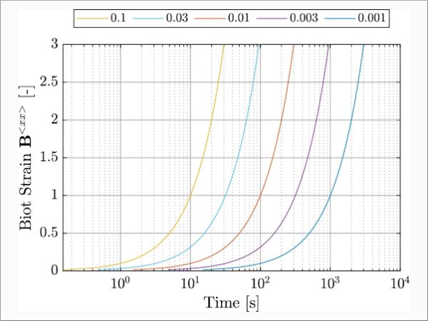
The subsequent section outlines the various test procedures, with all figures being presented on a logarithmic scale. These procedures encompass three distinct types of tests:

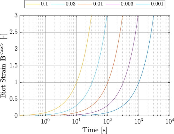
1. Tension tests until failure, depicted in Fig. 1.
2. Cyclic tests involving a loading and unloading cycle, illustrated in Fig. 2.
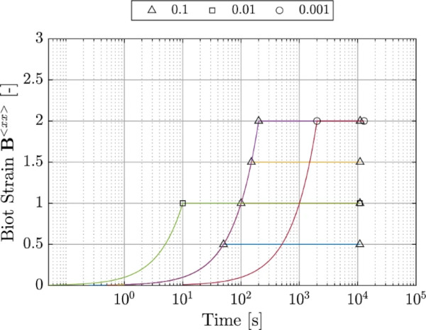
3. Relaxation tests, represented in Fig. 3.

The graphical representation in Fig. 1 provides a clear visualization of the applied strains over time for the experiments conducted at five different strain rates (0.1, 0.03, 0.01, 0.003, 0.001 [1/s]) until failure. It’s worth noting that a logarithmic scale is chosen to enhance precision and clarity. For ease of representation, the curves in Fig. 1 are presented up to a strain level of 300 [%]. It is essential to emphasize that no specific strain limit was defined within the test specification. The procedure was continued until the specimen reached the point of failure. As only the intact material behavior is considered in the following, there was no detailed evaluation of the failure.

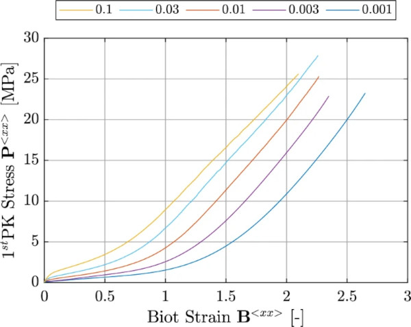
Figure 2 outlines the specific protocols employed for the cyclic tests. These tests were conducted with the primary aim of elucidating the size and configuration of the respective hystereses. Our investigation encompassed three distinct strain rates (0.001, 0.01, and 0.1 [1/s]). For each strain rate, the turning point of the hysteresis was set at a strain level of 150 [%]. For the test at a strain rate of 0.01 [1/s], we examined the hysteresis behavior at additional strain levels (50, 100, and 200 [%]). The tests were intentionally concluded when a force of 1 [N] was achieved to ensure that the specimens remained consistently under tension throughout the testing process.

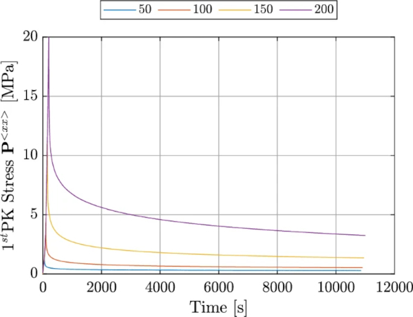
Figure 3 shows the different experimental procedures for the relaxation tests. The test specification for the relaxation tests encompasses a total of six distinct procedures. These procedures comprise two different strain rates (0.1, and 0.001 [1/s]), applied to two specific strain levels (100, and 200 [%]), and a third strain rate (0.01 [1/s]) at four various strain levels (50, 100, 150, and 200 [%]).

3.2 Results

The experimental procedures encompassed three distinct methodologies: tensile tests until failure, cyclic tests, and relaxation tests, all conducted in uniaxial stress state. These tests were executed with varying strain rates and loading durations to comprehensively assess the material’s mechanical response.

The subsequent sections present the results of each procedure. To maintain clarity and precision, we exclusively report the mean values derived from a minimum of three test iterations. This approach ensures that the presented results are representative and indicative of the material’s behavior under the specified testing conditions.

3.2.1 Tests until breakage

To investigate the rate dependency of standard PVB, uniaxial tensile tests were carried out at five different strain rates (according to the test specification, shown in Fig. 1). The observed material behavior can be divided into three sections. The first section contains an initial stiffness that increases with increasing strain rate. It follows a region of low stiffness, comparable to a flow plateau. A specific stress above which there is a sharp increase in the stress–strain relationship limits this section. Due to the greater initial stiffness concerning the higher strain rate tests, the stress increase occurs at locations of different strains. The area of sharp stiffness increase (3rd section) is almost parallel for all strain rates. Figure 4 shows the test results for five different strain rates until the failure of the specimen (0.001, 0.003, 0.01, 0.03, and 0.1 [1/s]).

3.2.2 Cyclic tests

In the context of the cyclic tests, it’s important to highlight that the specimens were subjected to loading and unloading phases using the same strain rate. Notably, a discernible dissimilarity between loading and unloading behaviors was evident. Furthermore, it became apparent that the hysteresis increased with increasing strain rates. This observation suggests that more energy is dissipated for higher strain rates.

Figure 5 shows the test results for strain rate 0.01 [1/s] and the strain levels 50, 100, 150 and 200 [%].

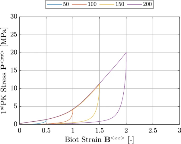
Figure 6 shows the results for three different loading rates (0.001, 0.01, and 0.1[1/s]) at a strain level of 150[%].

3.2.3 Relaxation tests

We investigated the relaxation behavior at different strain levels, applied with different strain rates. For all configurations we observed a very steep loss in stiffness at the beginning, followed by an almost horizontal course.

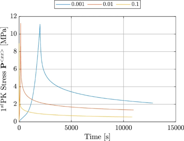
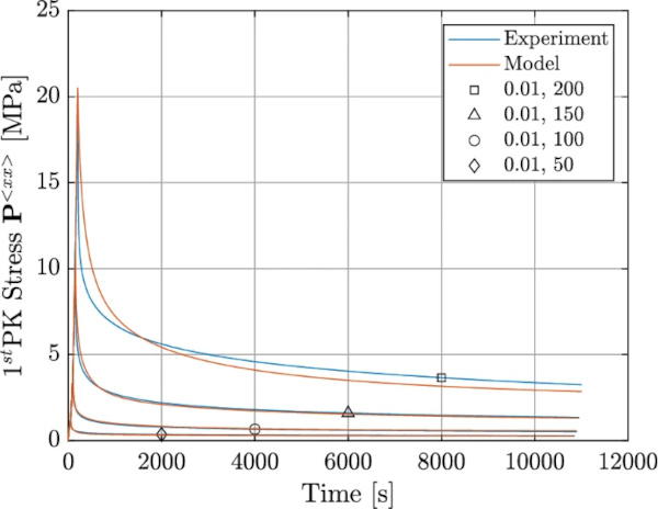
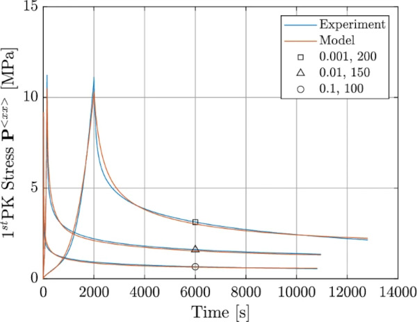
Figure 7 shows the test results for a strain rate of 0.01 [1/s] at 4 different strain levels (50, 100, 150 and 200 [%]), Figure 8 shows the results for the strain rates 0.1, 0.01, and 0.001 [1/s], along with the corresponding strain levels 100, 150, and 200 [%].

4 Modeling

This chapter serves as an introduction to the mechanical material model, which constitutes the primary focus of this study. It is subsequently followed by the process of identifying the relevant material parameters and conducting simulations of the presented tests.

4.1 Model construction

The model employed in this study adopts a phenomenological approach, setting it apart from the thermoplastic models presented in Sec. 1.3, which follow micromechanical considerations. It is founded upon the general framework for finite viscoelasticity, developed by Lubliner (1985), further adjusted by Haupt and Tsakmakis (1989) and implemented by Middendorf (2001). Notably, the model is extended to encompass compressible thermo-viscoelasticity while considering isothermal processes, a feature drawn from the work of Heimes (2004); Justine (2008).

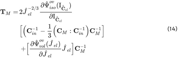
Diverging from models delineating the behavior of elastomers, such as those proposed by Lion (1996); Bergström and Boyce (1998); Middendorf (2001); Heimes (2004); Scheffer (2016), this model notably does not encompass an equilibrium stiffness component. Consequently, the material resistance in this model tends toward zero for infinitely prolonged processes. The formulation of the stress is depicted in Eq. 14.

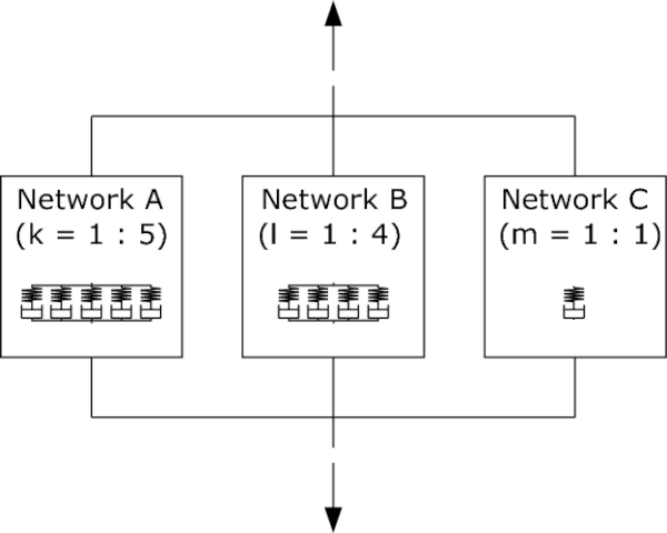
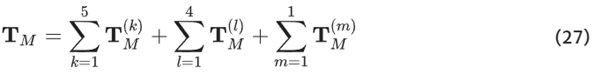
Following the designation proposed by Bergström and Boyce (1998); Boyce et al. (1988, 2000), the model is composed of three distinct networks: Network A, B, and C. Each network is characterized by its unique viscosity function. Networks A and B are rooted in the well-established Neo-Hookean potential, while Network C is anchored in the Yeoh potential. Both potentials are computationally robust and efficient. Network A represents the initial, rate-dependent stiffness, network B the material behavior over long time durations, network C the decisive hardening within the regime of large deformations. The viscosity functions within the model are characterized by different relaxation times and incorporate internal process variables (cf. Lion (1996); Reese and Govindjee (1998); Sedlan and Haupt (1999)) and stress barriers, a feature that aligns with the approach proposed by Lion (1996) to facilitate the rapid decay of initial stiffness. 

Additionally, a scalar-tensor function enhances viscosity at increasing strains, following the work of Sedlan and Haupt (1999); Lion (2000). The individual relaxation times are classified into several decades to ensure a smooth progression across a broad time scale. A further key element in the model’s material response is the utilization of a signum function, dependent on the strain rate, to differentiate between loading and unloading behaviors. This procedural concept was initially recommended by Bergström (1999). Furthermore, temperature dependency is introduced through the incorporation of a temperature-dependent viscosity parameter denoted as η₀, as outlined in the works of Holzapfel (1996); Lion (2000); Heimes (2004). This parameter plays a crucial role in capturing the impact of temperature variations on the material’s behavior, adding an essential thermomechanical aspect to the model. It is implemented in every network.

The model structure, as described earlier, serves as the fundamental framework for each of the networks. However, it’s important to note that in certain instances, this structure is subjected to modifications. Consequently, we provide individual and detailed descriptions for each of the networks in the following sections.

1. Network A: The elastic response is defined by the Neo-Hookean potential.

In the context of our multi-network model, Network A exhibits a sophisticated viscosity function (cf. Eq. 16), underpinned by several key components. First and foremost, a scalar tensor function is employed to gradually amplify viscosity as strains intensify. Complementing this, an additional exponential function, coupled with a stress barrier mechanism, has been integrated into the model. This mechanism introduces a stress threshold that, when surpassed, leads to an exponential decrease in viscosity (Lion 1996). This dynamic response faithfully mirrors the rapid decrease of the initial stiffness. To further enhance the model’s accuracy, a signum function is incorporated. This function effectively decouples loading and unloading behavior, a crucial element for capturing the observed hysteresis behavior. Finally, a secondary exponential function is introduced to capture the varying relaxation times observed during unloading (Scheffer 2016).

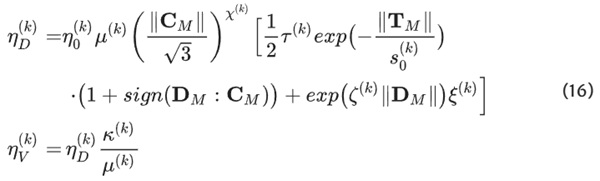
The total network A results in:

2. Network B: Much like Network A, the elastic response adopts the Neo-Hookean potential.

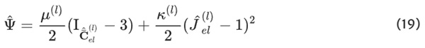
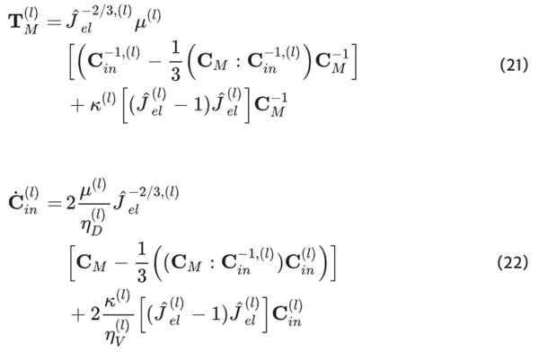
Within the viscosity function of Network B (cf. Eq. 20), a scalar tensor function is employed to closely align viscosity with changes in strain. Similar to Network A, Network B also embraces the inclusion of a signum function which serves the crucial purpose of distinguishing between loading and unloading phases. To further enhance the model’s accuracy, Network B introduces a secondary exponential function (Scheffer 2016). This function is dedicated to addressing the variations in relaxation times that the material exhibits during unloading.

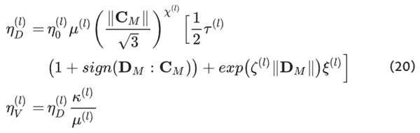
The total network B results in:

3. Network C: It introduces a distinctive departure by adopting the modified Yeoh potential, setting the coefficients C₁₀ and C₂₀ to zero (cf. Scheffer (2016)). This choice was made to uncouple the responses of Network A and B from the reaction of Network C within the regime of small to moderate strains.

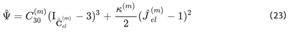
First and foremost, the viscosity function of Network C (cf. Eq. 24) leverages a scalar tensor function, strategically employed to incrementally amplify viscosity as strains escalate. Consistent with the principles employed in Networks A and B, Network C integrates a signum function within its viscosity formulation. It plays a pivotal role in distinguishing between loading and unloading phases, reflecting Network C’s commitment to modeling the nonlinear behavior exhibited by the material. Furthermore, Network C introduces a secondary exponential function to address the challenge of varying relaxation times that the material experiences during unloading. A noteworthy addition to Network C’s viscosity function is an extra term featuring an exponential function designed to reduce viscosity during relaxation processes markedly so as not to overestimate the response, as the relaxation time is chosen to be very long.

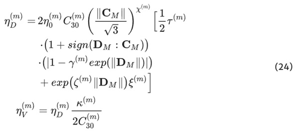
The total network C results in:

In summary, this multi-network model presents a powerful and adaptable framework for exploring the time- and temperature-dependent material behavior of PVB at large strains.

4.2 Parameteridentification

In this study, we have presented our experimental findings concerning PVB and introduced a mechanical model with the capability to provide qualitative predictions of the observed material responses. The model is contingent upon specific material parameters, thereby rendering it material-specific. It is imperative to optimize these parameters to establish a direct linkage between the empirical measurements and the model predictions. The optimization process is facilitated through an iterative algorithm. During each iteration, the model’s response is calculated by the experimental test specifications, and the resulting output is rigorously compared to the actual measurements. The comparison entails the computation of the error between the model’s predictions and the empirical data. These iterative calculations persist until the error is minimized, illustrating the crucial role of this iterative procedure in achieving an optimal alignment between the model and the empirical dataset.

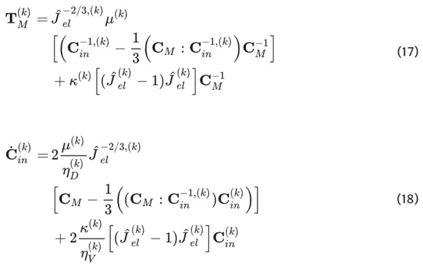
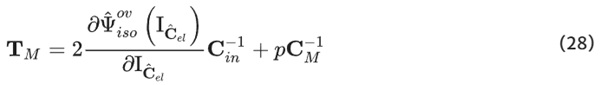
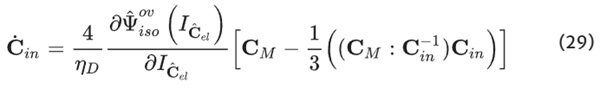
To speed up the numerical calculation, the three dimensional model, covering compressible material behavior, is simplified considerably. So far the energy and stress formulations are consequently separated into isochoric and volumetric parts. However, within this chapter the assumption of incompressible material behavior is applied and the deformation and stretch tensors are no longer separated into isochoric and volumetric parts. This assumption leads to a considerable simplification of Eq. 14. Furthermore, the volumetric part of the stress is replaced by the Lagrange multiplier p, representing hydrostatic pressure. In the end Eq. 14 is simplified to:

The flow rule stays in deviatoric form to ensure, that all inelastic deformations are of isochoric nature.

Furthermore, the model is reduced to the uniaxial stress state.

The first entry of the Second Piola Kirchhoff stress tensor

(uniaxial direction), based on a formulation in terms of invariants, yields:

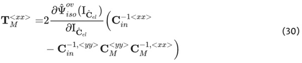
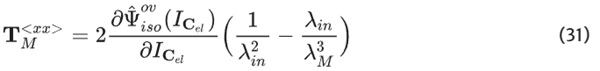
By inserting the principal stretches, Eq. 30, results in:

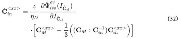
The first entry of the time derivative of the inelastic stretch stretch tensor 

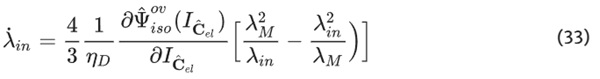
(uniaxial direction), based on a formulation in the terms of invariants, yields:

Inserting the principal stretches and solving for λ˙in yields:

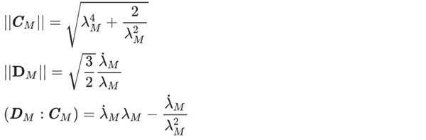
||CM||, ||DM||, and (DM:CM), formulated for the uniaxial case, yield:

Constructed on the reference configuration, the Second Piola Kirchhoff stress T must be transformed to the First Piola Kirchhoff stress P to compare it to the measurement results. This transformation rule reads P=FT

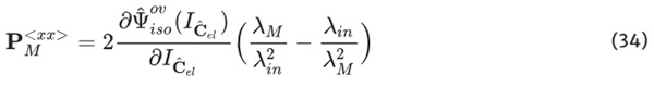
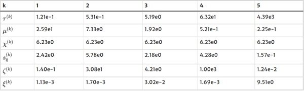
Table 1 Parameters of network A - Full size table

Considering that, all parameters are stored in the parameter-vector p=[p1;p2;p3], and the error function yields:

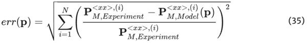
The optimization process involves the systematic variation of input parameters until the associated error reaches a minimal value. To identify the model parameters, we employed the global optimization algorithm “global search” (MATLAB), which incorporates the local solver “fmincon”. This local solver was already successfully utilized by Kuntsche (2015); Kraus and Niederwald (2017); Pauli and Siebert (2023). Given the substantial number of material parameters in the model, characterized by significant variations in magnitude, we applied a logarithmic transformation to these parameters to ensure a smooth adjustment during the optimization process.

Table 2 Parameters of network B - Full size table

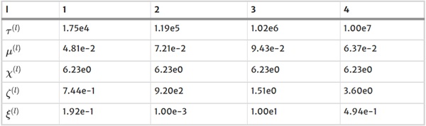
Table 3 Parameters of network C - Full size table

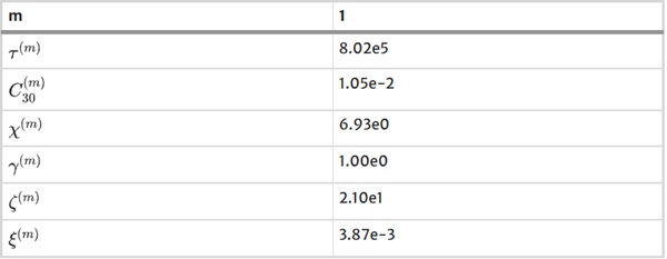
The optimization procedure unfolds in three distinct steps, sequentially forming the final parameter set, denoted as p. First, we calibrated the parameter set p₁=[τ;μ;C30;s₀;χ]ᵀ by utilizing results from the failure and relaxation tests. Subsequently, we calibrated parameter set p₂=[ξ]ᵀ using data from the failure, relaxation, and cyclic tests while keeping the already identified parameter set p₁ constant. Finally, parameter set p₃=[ζ;γ]ᵀ was calibrated using results from the failure, relaxation, and cyclic tests, while both parameter sets p₁ and p₂ remained constant.

Table 1, 2, and 3 present the final parameter sets tailored to the respective segments (networks) of the model. η₀ is equal to one for all networks.

4.3 Model calculation

The calculation results are compared with the measured data in the subsequent sections. This part is further divided into three distinct sections, each about the different types of tests: Tests until breakage, cyclic tests, and relaxation tests.

4.3.1 Tests until breakage

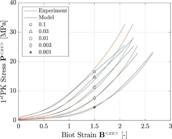
The comparison between the experimental data and the model calculations for the yield tests demonstrates an excellent agreement up to a strain of 150 [%] and a stress level of 20 [MPa], as shown in Fig. 10. Notably, for the highest strain rate of 0.1 [1/s] at higher strains, a maximum deviation of 20 [%] is observed. In general, it’s worth noting that the model’s response tends to be stiffer compared to the measured data.

4.3.2 Cyclic tests

The cyclic tests have been classified into two pairs. In the first group, these tests share a consistent applied strain rate (0.01[1/s]) but exhibit variations in their turning points (50,100,150,200[%]), where a “turning point” signifies the specific strain level at which the loading direction is reversed. Remarkably, the agreement between the test data and the model calculations is strong for the turning points corresponding to high strains (cf. Fig. 11). However, it’s important to acknowledge that the relative error tends to increase for turning points associated with smaller strains. Despite these variations, the model offers a qualitatively accurate representation of the overall behavior. Notably, the model captures the intricate shape of the hysteresis, illustrating the distinctive behavior during the transition from loading to unloading, even for scenarios involving significantly different strain levels.

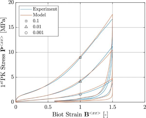
The second group of tests comprises those with a turning point occurring at the same strain level (150[%]) but with varying strain rates (0.001, 0.01,  and 0.1[1/s]). In these tests, the model calculations exhibit a high level of agreement with the experimental data, particularly for the cases with the highest strain rate. However, as the strain level decreases, the agreement becomes less accurate. Nevertheless, it’s important to note that the qualitative behavior is well-replicated within this second group, just as it was within the first group of tests (cf. Fig. 12).

4.3.3 Relaxation tests

Multiple relaxation tests were conducted and organized into two distinct groups. The first group comprises four tests, each corresponding to different strain levels (50, 100, 150, 200 [%]), all approached with a consistent strain rate of 0.01 [1/s]. It’s noteworthy that the strain levels of these relaxation tests align precisely with the turning points encountered in the cyclic tests. The modeling and experimental results for the first group are in excellent agreement (cf. Fig. 13).

The second group comprises three relaxation tests, each conducted at varying strain rates: 0.001,0.01,0.1[1/s] and each loaded to different strain levels, specifically 100, 150, and 200 [%]. Notably, the selection of these strain levels was designed such that the highest strain level was paired with the lowest strain rate, and so on. This approach was adopted to investigate the distinct response of the material for similar strain levels but under varying time histories. The relaxation tests conducted at various strain rates and levels, as shown in Fig. 14, also demonstrate excellent agreement.

5 Discussion

In the field of structural glass design, the predominant modeling approaches for describing the behavior of Polyvinyl Butyral (PVB) under large deformations have primarily revolved around hyperelasticity and finite linear viscoelasticity. Notable contributions in this area include the utilization of hyperelastic models by Kuntsche (2015); Kraus (2019); Pauli and Siebert (2023) and models of finite linear viscoelasticity Pelfrene (2016); Alter et al. (2017). However, Schuster (2023) made the first approach to describing the finite nonlinear viscoelastic phenomena of PVB utilizing the model developed by Schapery (1966, 1969).

The model we have presented in this work extends the considerations of linear viscoelasticity to finite deformations and incorporates nonlinear viscosity functions within the viscous flow rule. The comparison of the results of the model calculation and the presented experiments show a good match for different loading conditions, considering time dependency and large deformations. Moreover, although the focus of this work was on the time-dependent behavior at one particular temperature and humidity, the general formulation of the model provides for the incorporation of different temperatures considering isothermal conditions and can be expanded respectively. The model represents an important step towards a numerical model for the description of the residual load-bearing capacity, which marks a significant advancement in structural glass design.

Considering the actual structural design of the fully broken state of laminated glass, this material model could be implemented into a FEM (Finite Element Method) code or utilized inside analytical approaches. For a FEM implementation, the derivation of tangent operators within the three-dimensional model and the formulation of a User Material Subroutine (USERMAT) becomes an indispensable prerequisite. However, this derivation is beyond the scope of this paper. Considering idealized fracture patterns of laminates with coarse breaking glass (Kott 2007), relatively straightforward kinematic models (Seshadri et al. 2002; Belis et al. 2008) could suffice for the analysis of the residual load-bearing capacity. In this context, the presented model, simplified to one dimension, could be effectively employed. This utilization of our model holds the potential to provide valuable insights into such practical and relevant cases, offering a robust and versatile tool for advanced simulations.

Furthermore, in pursuing the overarching objective, the structural design of the fully broken state of laminated glass, establishing a robust failure criterion is paramount. This criterion can be equated with the failure of the interlayer or with a maximum deflection of the laminate causing failure of the whole structure. Considering the failure of the interlayer, the failure criterion is commonly defined based on principal strains or stresses. Throughout our analysis, a stress-dependent criterion emerged as a promising approach. However, it is essential to clarify that an extension of the investigated stress states, which was omitted in the current study due to the focus on temporal effects, becomes indispensable for formulating a specific failure criterion for the interlayer. However, this study lies beyond the scope of this current work.

6 Conclusion

In this study, we have developed a comprehensive finite nonlinear viscoelastic model to effectively capture the time-dependent behavior of Polyvinyl Butyral (PVB) at large deformations considering quasi-static loads. This model comprises a network of 10 Maxwell elements connected in parallel, with each element incorporating both a nonlinear damper and a hyperelastic spring. By utilizing viscosity functions with internal process variables, the dampers provide a robust and phenomenological description of the behavior of thermoplastic materials.

Our model’s calculations have demonstrated a commendable alignment between the experimental findings and the model’s predictions of PVB at a temperature of 20[∘C].

However, it is essential to consider certain aspects that require careful consideration. Despite the formulation that includes temperature effects, the model calibration was performed using data obtained under constant temperature and humidity conditions. To describe the material behavior at different temperatures, the presented tests would have to be carried out at these temperatures and considered for modeling and parameter identification. The parameter η0, an integral of each viscosity function, has not been considered yet. A respective formulation would have to be derived, expanding the model and the parameter identification. Furthermore, our investigation has been limited to the uniaxial stress state, and additional experiments would need to be conducted and included in the modeling and the parameter identification process for the precise modeling of different stress states. These aspects indicate possible avenues for further investigation and refinement in future research endeavors.

References

Funding

Author information

Ethics declarations

Additional information

Rights and permissions

About this article