Viscoelastic Fractional Model with a Non-Uniform Time Discretization for Laminated Glass: Experimental Validation

Article Information

• Digital Object Identifier (DOI): 10.47982/cgc.9. 619
• Published by Challenging Glass, on behalf of the author(s), at Stichting OpenAccess.
• Published as part of the peer-reviewed Challenging Glass Conference Proceedings, Volume 9, June 2024, 10.47982/cgc.9
• Editors: Christian Louter, Freek Bos & Jan Belis
• This work is licensed under a Creative Commons Attribution 4.0 International (CC BY 4.0) license.
• Copyright © 2024 with the author(s)

Authors:

• Lorenzo Santi - University of Parma
• Stephen Bennison - Kuraray America Inc, Wilmington DE
• Michael Haerth - Kuraray Europe GmbH, Troisdorf

Abstract

We discuss a novel approach, based on fractional calculus with a non-uniform time discretization, to numerically simulate interlayer viscoelastic behaviour and associated time-dependent deformation of laminated glass. Reference is made to the classic example of a simply supported laminated glass beam under long-duration loads. The fractional model is compared with some results obtained using the widely used finite element software ABAQUS 2021, which for the viscoelastic properties of the polymeric interlayer, utilizes the more traditional approach based on the Wiechert model and approximation via Prony series of the relaxation function and a uniform discretization of time for the numerical solution. The model is also validated through the comparison with the experimental test. 

The novel approach based on fractional calculus presents two main advantages: 1) the definition of the model parameters from experimental data is simplified; and 2) the numerical implementation is easier and computationally more efficient. When a long observation time is considered, the use of a non-uniform time discretization presents the great advantage of not neglecting any part of the relaxation function. The use of traditional uniform time discretization requires the use of large time steps making it impossible to describe all the changes of the relaxation curve within the large time interval. Practical examples will be presented using viscoelastic models for Trosifol® Extra Stiff (PVB) and SentryGlas® interlayers. This methodology also shows the potential to advance next-generation standards for the design of structural laminated glass. 

1.Introduction

Laminated glass is a layered structure composed of two (or more) glass plies bonded together by one (or more) thin thermoplastic polymeric interlayers, considered“flexible”. This means that the interlayers have no significant axial/flexural stiffness, and only provide shear coupling of the glass plies. The most used commercial interlayers are polyvinyl butyral (PVB), Ionoplast SentryGlas® (SG), and ethylene-vinyl acetate (EVA). Many variations of these materials exist depending on the number of plasticizers and metal salt added and the type of processing (M. Martin, 2020). In most design calculations the quasi-elastic approximation is followed, where the polymeric film is considered linear elastic, with an effective shear modulus calibrated on the duration of applied actions and operating temperature, which coincides with the secant value in relaxation tests. This is a simplified approach widely used in Standards and suitable for engineering approaches. However, when impulsive actions are applied (impact, blast waves), or when laminated glass is permanently strained as in cold bending and cold lamination bending, and more generally when the load is not monotone, the hereditary memory of viscoelasticity, neglected in the quasi-elastic approximation, may play a significant role (L. Galuppi, 2013). In such cases, a full viscoelastic analysis is required. The interlayer capacity of coupling the glass plies varies between the upper limit of fully coupled glass plies (monolithic limit) and the opposite lower limit of free-sliding plies (layered limit). The viscoelastic materials provide a condition that varies in time within these two limit cases.

The classical way to interpret the relaxation function of a polymeric material is through the Prony series based on the Maxwell-Wiechert model, which is the most general model for linear viscoelasticity (L. Biolzi, 2020). It takes into account that the relaxation does not occur at a single time, but in a set of times, so the relaxation curve is represented as a summation of exponential terms modeled as spring-dashpot elements in parallel each with a different decaying time and a single spring which is the stiffness of the material for times that tends to infinity (when all the dashpots are totally relaxed). However, experiments on a wide class of materials and, particularly, on most commercial polymers used as interlayers, indicate that the relaxation function can be well approximated by branches of power laws of time (L. Viviani M. D., 2023).

In a bi-logarithmic plot of the secant shear modulus vs. time, these correspond to a polyline, each segment of which is completely described by two parameters, i.e., its slope and the intercept with a vertical axis. When the relaxation function of a viscoelastic material is described by power laws, it is very effective to use rheological models based on fractional calculus. A fractional derivative is a derivative of any arbitrary order, real or complex, whose form coincides with Boltzmann’s convolution integral when the relaxation function is a power law. The numerical approximation of fractional derivatives can be performed via the Grünwald-Letnikov approximation (R. Scherer, 2011), which is very efficient since it provides the direct construction of a triangular matrix that operates on the discretized array of values of the relevant variables, which can be readily inverted. However, one of the major drawbacks of this method is that it is based on discretization in constant time steps: when the interval of observation is wide, too many steps would be needed to describe the long-term response. On the other hand, enlarging the time step results in a loss of accuracy.

What proposed here is an alternative numerical implementation of the viscoelastic model based on fractional calculus, according to which the approximation of the fractional derivates uses the L1 formula (R. Fazio, 2018). This allows for a variable time step, which increases in time to properly describe all the parts of the relaxation function (L. Santi G. R.-C., 2024), (L. Santi G. R.-C., 2024). 

2. Polymeric interlayer relaxation function

The viscoelastic behaviour of the materials used as interlayers can be described by their relaxation function. It is the long-term creep response of the material that indicates the stiffness’s time increasing. The relaxation function, for the interlayer, is experimentally obtained by prescribing a constant strain and measuring the stress decrease, i.e., the decay in time of the secant elastic modulus of the homogeneously strained specimen, or via oscillation experiments and TTS (DMA approach according to En16613). Structural modelling usually relies on Boltzmann’s superposition principle (linear viscoelasticity) and requires, as input datum, the relaxation function of the polymer.

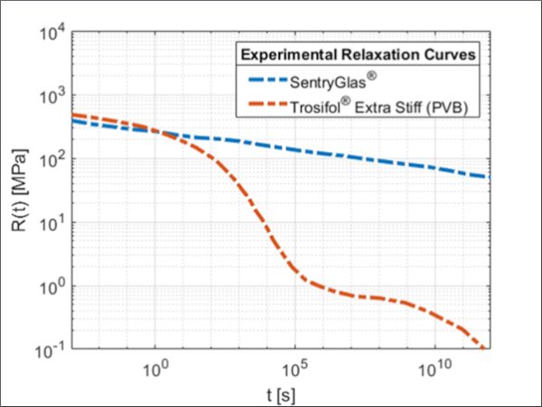
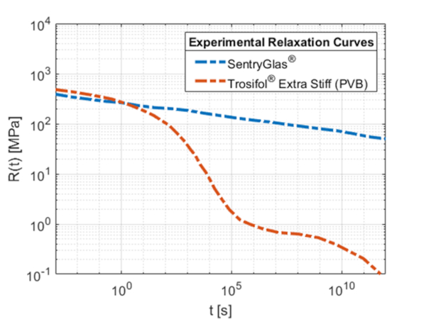
In the case of the laminated glass beam, the relaxation curve represents the coupling capability of the polymeric interlayer in time. In Figure 1 are represented the experimentally obtained relaxation curves of two commercial materials as a function of time: Trosifol® Extra Stiff (PVB) indicated with the red line and SentryGlas® indicated with the blue line obtained at the environmental temperature of 20o C with Dynamic Thermal Mechanical Analysis (DTMA). The experimental curves are provided by Kuraray GmbH, which also manufactures the interlayers (M. Schuster, 2023). The relaxation function’s qualitative trend of these materials is also published in (X. Centelles, 2021). It is possible to notice that, in the beginning, the two materials have similar stiffness, but over time the stiffness of Trosifol® Extra Stiff (PVB) significantly decreases, instead in the case of SentryGlas® it is much higher than the first material. This kind of behaviour is common for all the PVB types, and the effect of this property on the laminated glass will be evident in the following sections. Trosifol® Extra Stiff (PVB) and SentryGlas® are recalled Stiff PVB and Ionomer in the following for brevity.

The same curves are obtained in other experimental campaigns as shown in (X. Centelles, 2021), (L. Viviani M. D., 2023). 

2.1. The Prony series approximation

The classical way to interpolate the trend is through Prony series, which is a summation of exponential terms of the form 𝑅𝑖𝑒−𝑡 𝜗⁄𝑖, where 𝑅𝑖 is the i-th relaxation shear modulus, and 𝜗𝑖 the corresponding relaxation time. This series interprets the Wiechert model of viscoelasticity, which consists of an array of Maxwell units in parallel with a spring of stiffness 𝑅0, which represents the residual stiffness of the viscoelastic material when time tends to infinity (A.V. Duser, 1999). Consequently, the relaxation function reads: 

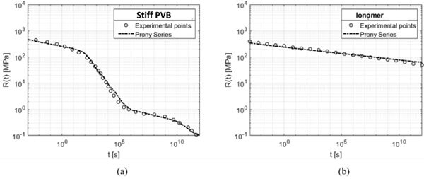
Figure 2 represents the approximation of the curves shown in Figure 1 for the two materials obtained using 11 terms of the series, this implies that 23 parameters need to be calibrated. A practical method, that has been used in this paper, to calibrate the coefficients is the Domain of Influence method (Bower, 1997), but its application is not straightforward, because the parameters are not supported by a geometric interpretation. On the one hand, a good fitting can only be obtained for a finite interval of observation: the longer this is, the higher the required number of terms in the Prony series. A similar procedure and fitting for a polymeric relaxation curve are also obtained in (S. J. Bennison, 1999). In Table 1 is represented the Prony series coefficients used to approximate the relaxation function of the two interlayers.

Table 1: Parameters 𝑅0, 𝑅𝑖 and 𝜗𝑖, defining the relaxation function in terms of Prony series, for Stiff PVB and Ionomer at 20°C. 

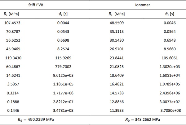
In the article (DIBt, 2022) are reported the Stiff PVB’s Prony parameters at the same temperature. It is possible to notice from the table in the paper, those parameters present some small differences because they have been calculated for a different observation period and using a different number of parameters in the Prony series, but the qualitative trend of the relaxation curve is the same.

2.2. Fractional derivatives approximation

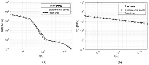
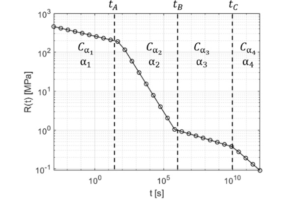
The shape of the relaxation function suggests that another feasible interpolation can be obtained with continuously connected branches of power laws, each one of the forms 𝐶_𝛼𝑡^−𝛼, with 0 <𝛼<1 (L. Viviani M. D., 2023). In the bi-logarithmic plot a power law corresponds to a straight line, this means that the curves of Figure 1 shall be approximated by a polyline composed of four segments, as indicated in Figure 3, where is represented as an example the material Stiff PVB. Each segment is defined by 2 parameters: the slope 𝛼 of the line and 𝐶𝛼 [𝑀P𝛼𝑠^𝛼], representing the stiffness value at 𝑡=1 𝑠. When the relevant interval of observation for the phenomenon is reduced, or in the case of the Ionomer where the curve can be easily approximated with only one power law, it can be sufficient to consider fewer branches.

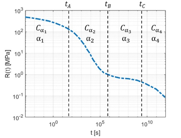
Table 2 presents the values of the coefficient of the power laws for each branch considered in the previous approximation. These values can be easily obtained through a linear interpolation of the graphs in Figure 1. This is a big advantage over the use of the Prony series approximation because to represent the relaxation curve we need less parameters, and they are also easier to calibrate.

Table 2: Coefficients that define the power-law approximation for the materials indicated in Figure 1.

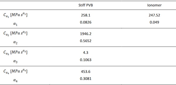
Figure 4 shows the representation of the two materials Stiff PVB (a) and Ionomer (b) through power laws, it is possible to notice that this approximation provides an excellent interpolation of the experimental points and it is accurate for most commercial polymers used as interlayers in laminated glass.

From the Stiff PVB’s relaxation curve is possible to notice some patterns that are typical for these kinds of materials used as interlayers. As investigated in (R. Alasfar, 2022), the curve, which has been divided in four different lines, presents some typical branches: 

• the first line, where the modulus is high, is called “Glassy region”. Here the polymeric interlayer presents a higher coupling capability between the glass plies.
• the second line is the “Glassy transition” where the negative slope of the line is higher, and the value of the relaxation modulus rapidly decrease in time.
• the third is the “Rubbery Plateau”, here the relaxation function settles on a lower value and do not decrease rapidly.
• the fourth is the “Viscous Flow” where the negative slope of the line increase and the material tends to not provide a high coupling between the glass plies due to a low value of the relaxation function.

Those branches are obtained analysing the time trend of the elastic shear modulus of the polymeric material at a fixed temperature, but they can be also obtained by varying the temperature in a small observation period. This property is at the basis of the William Landel Ferry model (M. L. Williams, 1955) which establishes a correlation between the time scale of the rheological phenomenon and the operating temperature. The response at other temperatures can be obtained by assuming the Time-Temperature Superposition principle (TTS), according to which any variation of the testing temperature is associated with a variation of the time scale for the effects of viscosity. Ionomer’s relaxation function doesn’t show those four different branches in this specific time interval even if the trend is decrescent, however also for this material, the curve tends to a lower limit value close to zero, at infinite load duration and temperature approaching its melting point. Experimental data at different temperatures are also available in the material’s portfolio (Kuraray, 2023), where it is possible to observe this lower plateau effect for high temperature.

The influence on the laminated glass structure’s deformation when the interlayer is in one of these different branches will be deeply analysed in the following sections.

There is a mathematical description of the equations of viscoelasticity founded on fractional calculus, because Boltzmann’s convolution integral coincides with the Caputo fractional derivative of order 𝛼𝛼when the relaxation function is expressed by a power law, as indicated as follows: 

However, to establish such a precise correspondence, it is necessary to formally write the power-law terms by defining the coefficients in terms of Euler’s Gamma function Γ, which is the generalization of the factorial n! to non-integer or complex values of n. In conclusion, the power-law approximation shown in Figure 3 of the relaxation function 𝑅(𝑡) takes the analytical form:

3. Simply supported beam model

The relaxation function described by branches of power laws with the fractional calculus will be applied to the model problem represented in Figure 5. This represents a simply supported three-layer beam, composed of two glass plies of thickness ℎ, bonded together by a thin polymeric interlayer of thickness 𝑠=𝑟ℎ, with 𝑟 ≪1. The Euler-Bernoulli beam has length 𝐿 and width 𝑏; the cross-sectional area of each ply is 𝐴=𝑏ℎ and the sum of the moments of inertia of the two plies is 𝐼=2·𝑏ℎ³/12, corresponding to the beam inertia at the layered limit. The total beam mass per unit length is 𝜇 [kg/m] and it is calculated by multiplying the glass density 2500 kg/m³ by the cross-sectional area 2A [m²] of the glass (the interlayer mass is neglected). A reference frame (y, z) is used as indicated in Figure 5. The beam is further subjected to the load per unit length 𝑝(𝑧,𝑡), variable in time. This model has been already analysed in (L. Viviani M. D.-C., 2022) (L. Santi G. R.-C., 2024).

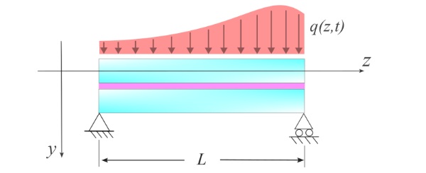
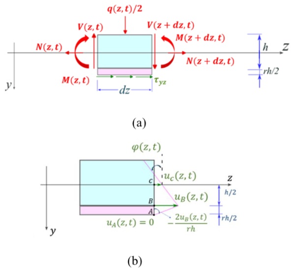
The interlayer is considered “flexible”, so its axial and bending stiffness is negligible, but it can provide the shear coupling of the glass plies, and it is supposed “thin”, so that the shear stress is constant in the thickness, although it can vary along the beam axis. Because of symmetry, it is sufficient to consider the equilibrium of the upper half of the beam (extrados ply plus half of the thickness of the interlayer), indicated in Figure 6a, for which 𝑉(𝑧,𝑡) is the shear force, 𝑁(𝑧,𝑡) is the axial force, 𝑀(𝑧,𝑡) is the bending moment and 𝜏𝑦𝑧(𝑧,𝑡) is the shear stress provided by the interlayer considered positive. Let 𝑣(𝑧,𝑡) denote the displacement of the point 𝑧 of the beam at the time 𝑡, considered positive in the 𝑦 direction.

According to Figure 6b, 𝜑(𝑧,𝑡) is the rotation of the cross-section, while 𝑢𝐴, 𝑢𝐵 and 𝑢𝐶 are the axial displacement of the points A, B and C, respectively. In the viscoelastic interlayer, from the Boltzmann superposition principle one obtains the constitutive equation takes the form:

In general, it is supposed that at 𝑡=0 the structure is undistorted, so that 𝜏𝑦𝑧(𝑧, 0)=0. If the relaxation function is a simple power law or a piecewise function of power laws as indicated in Equation 3:

Because of the definition of Caputo fractional derivatives indicated in Equation 2.

Considering the constitutive equation of the polymeric interlayer and the constitutive equation of the glass plies it is possible to write the governing equations of the system depending by the two unknows 𝑣(𝑧,𝑡) the vertical displacement and 𝑁(𝑧,𝑡) the axial force. It is necessary to separate the dependence on 𝑧 and 𝑡 to solve the system and thanks to an approach à la Galerkin it is possible to express the two unknowns through Fourier series that satisfy the boundary conditions (the axial force, the vertical displacement and its second derivative over 𝑧 are null for 𝑧=0 and 𝑧=𝐿). Also considering the initial conditions (the axial force, the vertical displacement and its first derivative in time are zero for 𝑡=0) it is possible to describe the system with one fractional differential equation with the vertical displacement as the only unknown (𝑣𝑛(𝑡) that depends only on time). The mathematical details of this treatment are reported in (L. Santi G. R.-C., 2024), (L. Viviani M. D., 2023) and (L. Viviani M. D.-C., 2022).

4. Numerical solution

To solve the fractional differential governing equation is necessary to approximate the Caputo fractional derivative. The classical method is through the Grünwald-Letnikov approach based on a constant subdivision of the observation time interval (R. Scherer, 2011). Another way is to use the so called L1 formula which allows a variable time step (R. Fazio, 2018), (S. B. Yuste, 2012). For this comparison has been preferred to use the second method because a variable subdivision of the time interval allows to not neglect any part of the relaxation curve, instead if a constant subdivision of time is used the time step become every large for big observation time, and it is not possible to describe all the changes of the curve within the time step. The advantages to use the second method instead of the first has been widely analysed within paper (L. Santi G. R.-C., 2024). The result of this is a better interpretation of the viscoelastic behaviour of the interlayer in time that brings a more accurate solution and less computational time in the numerical calculus. The use of a variable time steps allows also to compare the numerical solution with the widely used finite element software Abaqus that automatically implement a variable time step inside the solver to catch all the changes of the relaxation function.

4.1. The non uniform time discretization

To follow the long-term response, it is convenient to use a variable time step, which shall be small at the beginning, when the derivative of the relaxation curve is high, and large in the long run, when the relaxation curve tends to zero. Observing that each branch of power-law is a straight segment in the bi -log graph, it is natural to consider a discretized time vector such that log(𝑡𝑖+1)−log(𝑡𝑖)=𝑐=𝑐o𝑠𝑡, i.e., 𝑡𝑖+1=10𝑐𝑡𝑖, which corresponds to a constant interval in the bi-log graph. This partition, following a geometric progression, is shown in Figure 7. This choice is efficient and does not produce noteworthy errors, because the relaxation curve of a viscoelastic material is steepest at the beginning, where a dense time mesh is needed to capture all its variations, but becomes flatter over time, so that larger time steps can be used.

Figure 8 shows the time mesh in geometric progression for an observation time of 10¹² s with reference to a typical relaxation function interpolated by four branches of power law (Stiff PVB at 20°C). Observe that each branch is homogeneously represented, in the sense that the variation of the relaxation curve, in the bi -log graphs, is equally considered by the proposed partition.

The Caputo’s fractional derivative can be approximated through the L1 formula, that for a generic function 𝑓(𝑡) reads

Where 𝑅𝑛 is the local truncation error. The L1 formula can be easily applied to the vertical displacement and extended to a piecewise relaxation function composed by four temporal branches represented by power-laws, where the coefficients 𝛼 and 𝐶𝛼 vary in time as indicated in Figure 8. The total observation time is divided in 𝑠 intervals and each branch that compose the relaxation function contains a certain number of time intervals. Within a single branch the values of 𝛼𝛼 and 𝐶𝛼 remains the same. Also considering that

Approximating the fractional derivative with the L1 formula, It is possible to rewrite the governing equation of the system and solve it using a finite difference approach. It is important to mention that the equation is transformed in implicit form, this allows calculation of the vertical displacement at each temporal step. A more complete mathematical formulation of this treatment is published elsewhere (L. Santi G. R.-C., Variable time steps in the numerical implementation of viscoelastic fractional models for laminated glass, 2024). The complete solution is obtained by summing all the terms of the Fourier expansion, in this case, for a good approximation, is sufficient to consider the first non-null terms because they are dominant against the others.

4.2. Comparison through the fractional model and ABAQUS 2021

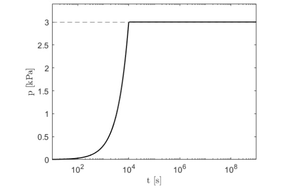
The algebraic equation is numerically solved with MATLAB. Consider, as a benchmark problem, the simply supported laminated glass beam. Set L = 1.5 m, b = 1 m, h = 8 mm, s = rh = 1.52mm(r = 0.19), E = 72 GPa, μ= 40kg/m. The deformation of the beam is evaluated by the mid-span displacement v(z/2, t). The structure is subjected to a uniformly distributed load varying in time as shown in Figure 9: this is a uniformly distributed pressure p(t) that starts from zero and linearly increases, reaching the plateau 3 kPa in approximately 1 hour. Consequently, the load per unit length is q(z, t)= b p(t) The interval of observation is chosen sufficiently long, of the order of 10⁹ s (approximately 3 years) to emphasize possible differences in the long-term creep response. The layered (monolithic) limit corresponds to free sliding (fully coupled) glass plies and is attained when Cα→ 0 (Cα→∞). The deflection at mid-span at the layered and monolithic limits can be evaluated as

respectively, which gives 32mm and 6.1mm when p(t) reaches the maximum value of 3 kPa.

The capacity of the polymeric interlayer to couple the glass ply can be qualitatively estimated by comparing the calculated value of v(L/2, t) through the resolution of the governing equation before mentioned with the monolithic and layered limits. In general, the stiffer the relaxation curve, the lower the displacement shall be, for example, referring to Figure 1, lower values of the vertical displacement with for Ionomer than Stiff PVB are expected.

The fractional viscoelastic model is validated via comparison with the results obtained with the commercial finite element software ABAQUS 2021 (ABAQUS/Standard User’s Manual, Version 6.9., 2021). This implements a full viscoelastic analysis based upon the solution of the integral-differential equations resulting from Boltzmann superposition principle, but it does not use the mathematical characterization via fractional calculus and the relaxation function can only be assigned as a Prony series of exponential terms, as shown in equation (1). The numerical solver uses a variable time-step of integration, which is automatically updated to minimize the temporal mesh for convergence. The beam structure has been modelled with 8-node solid elements, available in ABAQUS library. The glass is linear elastic, whereas the interlayer is a linear viscoelastic incompressible material, for which therelaxation function under shear is described by Prony series, the coefficients are reported in Table 2.

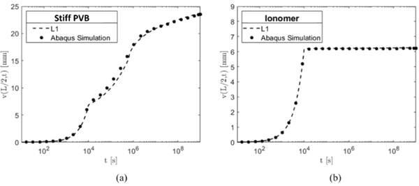
Figure 10 shows the comparison between the solution obtained through fractional differential equation indicated with dotted line (L1) and the finite element model in ABAQUS indicated with asterisks. The two solutions perfectly coincide and the error between them is lower than the 1% , this confirms the reliability of the new method based on fractional derivatives.

In the investigated time/temperature combination, the vertical displacement time history of the Ionomer does not show particularly strong viscoelastic effects because the interlayer is very stiff (at higher temperatures become visible), and its relaxation curve is different from the Stiff PVB’s that present a big drop in the trend. When the Ionomer is used as interlayer, the vertical displacement value is close to the monolithic limit (6.1 mm) and that underlines how this material gives stiffness to the structure comparable to a monolithic slab as shown in Figure 10b. A different behaviour of the vertical displacement time history is presented when the Stiff PVB is used as interlayer. From Figure 1 it is evident how the stiffness of this material diminishes in time in contrast to Ionomer and that aspect affects the response of the beam to a load, indeed from Figure 10a it is evident how the vertical displacement of the beam increases in time passing from a value close to the monolithic limit (“Glassy region”) to a value that tends to the layered limit 32 mm (“Viscous Flow”). Stiff PVB is an interlayer that don’t guarantee a constant stiffness of the layered glass beam for a long observation period, instead with Ionomer the structure has a behaviour comparable to a monolithic beam, for the investigated time/temperature combination.

4.3. Convergence analysis

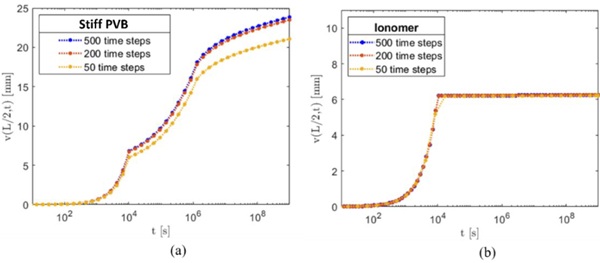
Figure 11 shows the convergence analysis for the solution of the fractional differential equation using the two materials as interlayer. Here, the number of time steps is varied and the difference in the solutions evaluated, the convergence is achieved when such difference becomes less than a target value, in our case we can see that, for Stiff PVB, the solution does not significantly vary if it is calculated with 200 time steps, instead if Ionomer is used, which is stiffer than the previous material, the convergence is reached with 50 time steps. This analysis confirms that the greater the stiffness of the material, the lower the number of time steps required to achieve convergence.

4.4. Comparison with experimental results 

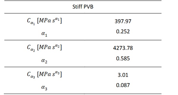
The fractional model of the laminated glass beam is compared with the results of an experimental campaign from (X. Centelles, 2021). The experimental setup is the same proposed in the previous numerical analysis: a simply supported laminated glass beam, with the same geometry, under uniformly distributed load of 3 kN/m2. The relaxation function of Stiff PVB, calculated in the experimental campaign, is interpolated with piecewise function of power laws as for the curves proposed in this article and the parameters are shown in Table 3, instead the coefficient for Ionomeris the same reported in Table 1. The Stiff PVB’s parameters, also reported in (L. Viviani M. D., 2023) for both materials, are slightly different from those in Table 1, because they are calculated for a different time interval and at a different temperature.

Table 3: Coefficients that define the power-law approximation for the material Stiff PVB from the curve presented in (X. Centelles, 2021) at the temperature of 23°C.

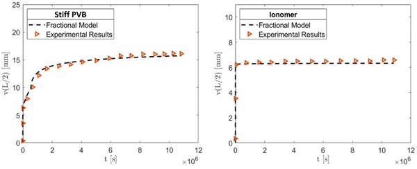
The solution reported in Figure 12 is calculated for an observation time around 107 seconds (four months). The numerical results match the experimental points with a good accuracy and the error between them is lower than 3%. Even in this case it is possible to observe the bigger stiffness that an interlayer as Ionomer can bring to the laminated glass structure, indeed also in this case, the maximum vertical displacement settles on the monolithic limit, instead using Stiff PVB the deformation monotonically increases in time due to a more pronounced decrease in stiffness in the material. This comparison prove how fractional formulation in the constitutive equation of the polymeric interlayercan well approximate its viscoelastic properties and allows to simulate experimental tests with a good precision.

5. Conclusion 

A numerical algorithm has been considered to calculate the long-term rheological response of laminated glass under varying applied loads, which supports a non-uniform discretization of the time interval of observation. This applies to viscoelastic models that are mathematically described via fractional calculus and are particularly efficient when the relaxation curve of the polymeric interlayeris represented by a power law, or continuously connected branches of power laws, as is the case of most commercial materials used in laminate glass. A time mesh of points spaced in geometric progression has been proposed, which corresponds to constant intervals in a logarithmic representation of time because, for a long observation period (109 seconds), no part of the relaxation curve is neglected. This choice fits with the assumed character of the relaxation function which, in a bi -logarithmic representation, corresponds to a polyline. The fractional derivative has been numerically approximated through the L1 formula because it supports a non-uniform time discretization, contrary to the classical Grünwald-Letnikov method. This new mathematical approach has been applied to the classical system of a simply supported laminated glass beam under uniformly distributed load. The vertical displacement trends for two different interlayer materials: Stiff PVB and Ionomer have been calculated.

This study confirms the reliability of the new approach because the numerical results has been compared with an ABAQUS simulation and the error between them is lower than 1%. It has also demonstrated the difference between the two interlayers studied: Ionomer is stiffer than Stiff PVB and this strongly affects the vertical displacements of the beam, indeed with the first material the solution almost coincides with the monolithic limit for the entire observation period, instead with the second material this happen only at an early stage and then the vertical displacement tends to the layered limit. This behaviour is expected from the relaxation curves of the two materials that shows how the Ionomer remains stiffer than the Stiff PVB for a longer period. The model is also validated with experimental results and the comparison show how the numerical solution can well describe the viscoelastic behaviour of the polymeric interlayer.

Acknowledgements

• Funder: Project funded under the National Recovery and Resilience Plan (NRRP), Mission 4Component 2 Investment D.M. - Call for tender No. 352 of DATE of Italian Ministry of 2022 funded by the European Union – NextGenerationEU
• Award Number: 38-033-21-DOT13SJY60-2678, Concession Decree No. 352 of DATE adopted by the Italian Ministry of 09/04/2022, D92B22000670005

References

A.V. Duser, A. J. (1999). Analysis of Glass/Polyvinyl Butyral Laminates Subjected to Uniform Pressure. Journal of engineering mechanics, 435-442, https://doi.org/10.1061/(ASCE)0733-9399(1999)125:4(435).
ABAQUS/Standard User’s Manual, Version 6.9. (2021).
Bower, F. G. (1997). Domain of influence method: a new method for approximating prony series coefficients and exponents for viscoelastic materials. Journal of Polymer Engineering, 1-22, https://doi.org/10.1515/POLYENG.1997.17.1.1.
DIBt. (2022). allgemeine bauartgenehmigung.
Kuraray. (2023). Product portfolio SentryGlas®.
L. Biolzi, S. C. (2020). Constituitive relationships of different interlayer materials for laminated glass. Composite Structures, 244, https://doi.org/10.1016/j.compstruct.2020.112221.
L. Galuppi, G. R.-C. (2013). The design of laminated glass under time dependent loading. International Journal of Mechanical Sciences, 67-75, https://doi.org/10.1016/j.ijmecsci.2012.12.019.
L. Santi, G. R.-C. (2024). Variable time steps in the numerical implementation of viscoelastic fractional models for laminated glass. Journal of Applied Mechanics, 1-21, https://doi.org/10.1115/1.4064433.
L. Santi, G. R.-C. (2024). Viscoelastic modelling via fractional calculus of the cold bending of laminated glass. Engineering Structures, 305, https://doi.org/10.1016/j.engstruct.2024.117756.
L. Santi, S. B.-C. (2023). Fractional viscoelastic modelling of polymeric interlayers in laminated glass, comparison with prony series approach. Glass Performance Days (GPD). Tampere: 85-89, .
L. Viviani, M. D. (2023). Piecewise power law approximation of the interlayer relaxation curve for the long-term viscoelastic fractional modeling of laminated glass. Composite Structures, https://doi.org/10.1016/j.compstruct.2023.117505.
L. Viviani, M. D.-C. (2022). A fractional viscoelastic model for laminated glass sandwich plates under blast actions. International Journal, https://doi.org/10.1016/j.ijmecsci.2022.107204.
M. L. Williams, R. F. (1955). The temperature dependence of relaxation mechanisms in amorphous polymers and other glass-forming liquids. Journal of the American Chemical Society, 3701–3707, https://doi.org/10.1021/ja01619a008.
M. Martin, X. C. (2020). Polymeric interlayer materials for laminated glass: A review. Construction and Buildings materials, https://doi.org/10.1016/j.conbuildmat.2019.116897.
M. Schuster, M. H. (2023). Quantification of the linear viscoelastic behavior of multilayer polymer interlayers for laminatedglass. Glass Structures and Engineering, 457-479, https://doi.org/10.1007/s40940-023-00229-w.
R. Alasfar, S. A. (2022). A Review on the Modeling of the Elastic Modulus and Yield Stress of Polymers and Polymer Nanocomposites: Effect of Temperature, Loading Rate and Porosity. Polymers, 14(3), 360; https://doi.org/10.3390/polym14030360.
R. Fazio, A. J. (2018). A finite difference method on non-uniform meshes for time-fractional advection–diffusion equations with a source term. Applied Sciences, 8(6), 960; https://doi.org/10.3390/app8060960.
R. Scherer, S. L. (2011). The grunwald–letnikov method for fractional differential equations. Computers and Mathematics with Applications, 902-917, https://doi.org/10.1016/j.camwa.2011.03.054.
S. B. Yuste, J. Q.-M. (2012). A finite difference method with non-uniform timesteps for fractional diffusion equations. Computer Physics Communications, 2594-2600, https://doi.org/10.1016/j.cpc.2012.07.011.
S. B. Yuste, J. Q.-M. (2016). Fast, accurate and robust adaptive finite difference methods for fractional diffusion equations. Numerical Algorithms, 207–228, https://doi.org/10.1007/s11075-015-9998-1. 
S. J. Bennison, A. J. (1999). Fracture of Glass/Poly (vinyl butyral) (Butacite®) Laminates in Biaxial Flexure. Journal of the American Ceramic Society, 1761-1770, https://doi.org/10.1111/j.1151-2916.1999.tb01997.x.
X. Centelles, F. M. (2021). Long-Term loading and recovery of a laminated glass slab with three different interlayers. Construction and Building Materials, https://doi.org/10.1016/j.conbuildmat.2021.122991.