Authors: Michael Drass, Hagen Berthold, Michael A. Kraus & Steffen Müller-Braun
Source: Glass Structures & Engineering | https://doi.org/10.1007/s40940-020-00133-7
Abstract
In this paper, artificial intelligence (AI) will be applied for the first time in the context of glass processing. The goal is to use an algorithm based on artificial intelligence to detect the fractured edge of a cut glass in order to generate a so-called mask image by AI. In the context of AI, this is a classical problem of semantic segmentation, in which objects (here the cut-edge of the cut glass) are automatically surrounded by the power of AI or detected and drawn. An original image of a cut glass edge is implemented into a deep neural net and processed in such a way that a mask image, i.e. an image of the cut edge, is automatically generated.
Currently, this is only possible by manual tracing the cut-edge due to the fact that the crack contour of glass can sometimes only be recognized roughly. After manually marking the crack using an image processing program, the contour is then automatically evaluated further. AI and deep learning may provide the potential to automate the step of manual detection of the cut-edge of cut glass to great extent. In addition to the enormous time savings, the objectivity and reproducibility of detection is an important aspect, which will be addressed in this paper.
Introduction
Cutting of glass

In the production and further processing of annealed float glass, the glass panes are usually brought into the required dimensions by a cutting process. In a first step, a fissure is generated on the glass surface by using a cutting wheel. In the second step, the cut is opened along the fissure by applying a bending stress. This cutting process is influenced by many parameters (Müller-Braun et al. 2020). The edge strength in particular can be reproducibly increased by a proper adjustment of the parameters (Ensslen and Müller-Braun 2017).
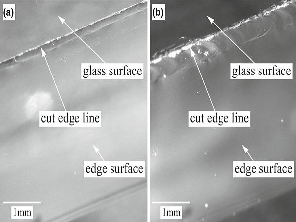
Furthermore, it could be observed that due to different cutting process parameters, the resulting damage to the edge (the crack system) can differ in its extent (Fig. 1). In addition, this characteristic of the crack system can be brought into a relationship with the strength (Müller-Braun et al. 2018). In particular, it has been found that when the edge is viewed perpendicular to the glass surface (Fig. 2), the so-called lateral cracks, which can be observed here, allow the best predictions for strength (Müller-Braun et al. 2020). The challenge here is to detect these lateral cracks in an accurate way.
Currently, this is only possible by manual tracing due to the fact that the crack contour can sometimes only be recognized roughly (Fig. 2). After manually marking the crack using an image processing program, the contour is then automatically evaluated further. Methods of Artificial Intelligence (AI) and especially the algorithms from the field of AI in computer vision may provide the potential to automate the step of manual detection as well. In addition to the enormous time savings, the objectivity and reproducibility of detection is an important aspect.

Artificial intelligence, machine and deep learning
In this section, we define the essential terms of Artificial Intelligence, Machine and Deep Learning in order to bring them closer to the reader. In case the reader is familiar with it, then this section should be skipped.
Artificial intelligence (AI) is the overall term for all subsequent developments, algorithms, forms and measures in which artificially intelligent action occurs. AI is dedicated to the theory and development of computational systems capable of performing tasks that normally require human intelligence, such as visual perception, speech recognition, decision making and translation between languages.
Machine learning (ML) is a sub-class of AI, which enables systems to learn from given data and not to execute or make actions, commands or decisions by explicit programming. The aim of ML is to generate artificial knowledge from experience (the data). A basic premise, however, is that the knowledge gained from the data can be generalized and used for new problem solutions, for the analysis of previously unknown data or for predictions on data not measured (prediction) (Kraus 2019b; Bishop 2006). Excellent examples for classical machine learning are linear classifiers (e.g. linear/logistic regression, linear discriminant analysis), kernel methods (e.g. support vector machines), tree-based methods (e.g. decision trees, random forests), non-parametric regression (e.g. nearest neighbors, local kernel smoothing), etc. (Kraus 2019a; Kraus and Drass 2020b).
Deep neural networks (DNN) or Deep learning uses so-called artificial neural networks to recognize patterns and highly non-linear relationships in data. A deep neural network (DNN) is based on a collection of connected nodes (the neurons), which fictitiously resemble the human brain (cf. Fig. 5). Due to their ability to reproduce and model nonlinear processes, deep neural networks have found applications in many areas (Voulodimos et al. 2018). These include material modeling and development, system identification and control (vehicle control, process control), pattern recognition (radar systems, face recognition, signal classification, 3D reconstruction, object recognition and more), sequence recognition (gesture, speech, handwriting and text recognition), medical diagnostics, social network filtering and e-mail spam filtering.
To give the interested reader an even better introduction to the application of Artificial Intelligence in practical relation to structural glass engineering and processing, we refer to the current review article proposed by Kraus and Drass (2020a).
Problem statement and methodology
The problem is defined, whether it is possible with the help of AI to firstly recognize the fracture pattern of a cut glass edge and secondly to process it in such a way that AI automatically creates an image, so-called mask image of the cut edge, without explicitly programming it.
Methodologically, this problem is to be solved with the help of so-called semantic segmentation using deep convolutional networks. This method is preferred because it has wide application for describing and solving image segmentation problems. Image segmentation means creating a contour plot around a specific object, such as a ball, in an image. The goal here is to automatically generate a high-resolution image of the fracture pattern of the cut glass edge, which can be used later to perform statistical analysis regarding the characteristics of the cut glass edge.
Since in this paper, it is the first time that AI algorithm are applied to a specific problem of glass processing, Chapter 2 gives a brief introduction into AI and deep learning. Since we want to focus on the problem of semantic segmentation in this paper with the help of Deep Learning, i.e. the task of classifying each and very pixel in an image into a class (here cut glass edge), we will introduce semantic segmentation briefly in Chapter 3. Chapter 4 will then deal specifically with the task of semantic segmentation using images of cut glass edges to determine the contour of the broken edge.
Fundamentals on deep learning
This section aims at explaining deep learning and summarizing its main features to help the reader understand the algorithms that follow. In case one is familiar with Deep Learning, this section can be skipped.
To understand how a neural network works, the example of a so-called multi-layer perceptron (MLP) is explained below. An MLP consists of at least three node layers: an input layer, a hidden layer and an output layer. Within the layers there are neurons, each with different tasks. With the exception of the input nodes, each node is a neuron that uses a nonlinear activation function. For training, MLP uses a technique of supervised learning called backpropagation to adjust the weights w of the neural network. An MLP is hence a mathematical composition of nonlinear functions of two or more neurons via an activation function.
This particular nonlinear nature of NNs thus is able to identify and model nonlinear behaviors, which may not at all or not properly be captured by other ML methods such as regression techniques or PCA etc. Despite the biological inspiration of the term neural network a NN in ML is a pure mathematical construct which consists of either feedforward or feedback networks (recurrent). The neurons at the outputs are called output neurons, the layers in between the input and output neurons are called hidden layers. If there are more than three hidden layers, this NN is called a Deep NN. The development of the right architecture for an NN or Deep NN is problem dependent and only few rules of thumb exist for that setup (Bishop 2006; Frochte 2019; Kim 2017; Paluszek and Thomas 2016).
To describe the structure and mathematical processes of an NN during learning (training), the example of handwriting recognition based on the MNIST dataset is used for reasons of comprehensibility. This is about predicting the written numbers (0–9) based on input images without writing an explicit algorithm doing that task. The MNIST database contains 60,000 training images and 10,000 testing images. An example of several input images is summarized in Fig. 3. Each single image has a resolution of 28×28 pixels, which are then used as input within the NN.

Therefore, the first layer of the NN consists only of the image data, which is fed into the network as initial information. It is to note that the input image is not read in as an image but as a vector x with a length of 28×8=784. The values within the input vector of each image is the corresponding gray value of the image. Each value in the input layer corresponds in the context NN to a single input neuron, which in turn is connected to all following neurons of a hidden layer. The last layer in NN is the so-called output layer. In this output layer, NN makes a prediction with respect which number was identified in a corresponding input-image. A typical NN architecture for the problem of handwriting image recognition is displayed in Fig. 4.

As can be seen in Fig. 4, the input vector x has 784 entries, each of which is connected to the neurons of the hidden layer. The output layer is defined as a vector that has exactly 10 entries and predicts the handwriting recognition solution. To understand more precisely how the training of a neural network works, only one neuron of the first hidden layer is shown in the following figure.

Each neuron receives a set of values (numbered from 1 to i) as an input and compute within the hidden layers activation signals a as output. In the final layer, the output layer, the neurons compute the predicted y^ value. The vector x actually contains the values of the features in one of m examples from the training set. Just to remember, the MNIST dataset contains 60,000 training images, hence m is equal to that number. In addition, each unit has its own set of parameters, usually referred to as w (column vector of weights) and b ( bias), which change during the learning process. During each iteration, the neuron computes a weighted average of the values of vector x, based on its current weighting vector w, and adds a bias b. For each neuron of the hidden layer, the weighted average is calculated as
![]()
Finally, the result of this calculation is passed through a nonlinear activation function called g. Activation functions are one of the key elements of the neural network. Without them, our neural network would become a combination of linear functions, so it would itself be only a linear function. After the first feed-forward run through the NN, a so-called loss function must be computed. The basic source of information about the state of learning is the value of the loss function. In general, the loss function should show how far from the “ideal” solution a person is. Since there are many different functions for describing the loss function L, the mean absolute value of the loss function J is generally described by

At this point it should be noted that all neurons of all hidden layers are now considered, so that a matrix of weightings W is calculated from the weighting vector of a single neuron. The scalar of bias b is now also turned into a vector b for all neurons. For the calculation of the mean absolute value of the loss function J all images with the number m are used. The index i corresponds to the length of the input vector x, so the loss function L is a function of the calculated predictor y^i and the true value yi.
Now that the loss function is defined, and we have arrived at the output of NN in the first iteration of the feed-forward procedure, we have to minimize the loss function by adjusting the matrix of weightings W and the bias vector b. For this purpose, calculus will be used for help and the gradient descent method will be applied to find a functional minimum. Throughout each iteration the value of the partial derivatives of the loss function with respect to each of the parameters of the neural network will be computed. The adjusted parameters of the neural network are computed with
![]()
and
![]()
In the above equations, the learning rate is represented by α which is a hyper parameter that allows the user to control the value of the adjustment performed. Choosing the learning rate is essential—if it is too low, the NN learns very slowly, if it is too high, the NN cannot reach the minimum. dW and db are calculated using the chain rule, partial derivatives of the loss function with respect to W and b. The size of dW and dbbdbb is the same as that of W and b, respectively. Figure 6 shows the sequence of operations within the neural network. It clearly shows how forward and backward propagation interact to optimize the loss function (Fig. 5).


Semantic segmentation with deep learning
Today, in the context of computer vision and deep neural networks, the topic of image classification is widely known. Typically, in image classification one tries to classify images based on its visual content. For instance, the classification algorithm of an image can be designed to detect whether an image contains a car, animal, point fixing for facades, etc. or not. Whilst the recognition of an object is trivial for humans, for computer vision applications, robust image classification is still a challenge. An extension of this deals with so-called object detection, in which objects within an image are enclosed by a frame or box.
Regarding the accuracy of the resolution of object detection, it is relatively coarse, so in some cases it is desirable to detect the exact contours of objects. Considering semantic segmentation in contrast, it is the task of classifying each individual pixel in an image into a specific class. Typically, in the task of semantic segmentation, image data is read in and evaluated in such a way that an object to be found is segmented or bordered by a so-called mask. An example of the algorithms listed above is shown in Fig. 7 for the example of the detection of point fixings in a facade.
In summary, one can say that the greatest information content in an image classification problem is obtained via semantic segmentation. In the past it has been shown that especially in image classification neural networks have become established, because they are very well able to recognize (hidden) patterns in images. These hidden patterns can be named also as features, which should be recognized and learned by the neural network in order to make robust predictions on the input images.
Semantic segmentation on cut-edge of glass
In the following, the method of semantic segmentation is applied to images of cut edges of glasses. The aim is to detect and trace fracture edges of images of cut glass using the method of semantic segmentation. With the successful application of this method it will be possible in future to statistically evaluate images of broken glass edges in terms of the fracture pattern, crack branching system and their crack width without having to invest a lot of time in image processing and post-processing, which was very time-consuming in the past.
Data: original input–output
The object of interest are conventional 8 mm thick annealed Soda-lime glass panes, which were industrial cut using a classical carbide cutting wheel. The edges of these panes were photographed perpendicular to the glass surface, with the edge always positioned in the centre of the image (Fig. 8 (top)). Accordingly, this procedure always ensures the same boundary conditions when capturing the images of the cut edge. The input images were taken with a camera with the model number U3-3890CP-M-GL Rev.2 from IDS Imaging Development Systems GmbH. This camera has a monochrome sensor with a resolution of 4000×3000 px. As lens the LM25JC10M of the company Kowa Optimed Deutschland GmbH was used. With a focal length of 25 mm, this allows macro photography with a minimum distance of the object to the lens of 100 mm.
Thus, a very high level of detail could be realized with a relatively large image section at the same time. The scale of the input images is 1/8.696 px/μμm. For the illumination a homogeneous white LED transmission light with the model code TH2-63X60SW from CCS Inc. (OPTEX GROUP CO., LTD.) was used together with the Digital Control Unit PD2-3024(A). The images were taken with the lowest brightness level. For further processing, the file size of the images was reduced by trimming the upper and lower 1250 px, as the image information in these areas are irrelevant for the investigations. Thus, image files with a size of 4000×500 px were generated.
In a further step, the visible lateral cracks were marked manually using the image processing program Adobe Photoshop. The crack contour was first traced with a 1 px thick line. Afterwards a 1 px straight line was positioned at the edge of the glass pane. Finally, the resulting space between the two lines was filled with black. The result is the output mask shown in Fig. 8 (bottom).

This kind of processing of the individual input images is very tedious and time-consuming, so the goal is to develop an automatic generation of mask images via AI.
Data: preparation and augmentation
Data preparation
The database is formed by four images with a pixel size of 500 ×× 4000 px. The color space has already been reduced manually to only have gray values within the images. From the previous investigations it became clear that a square section of 192 × 192 px is a sufficient dimension to represent the size we are looking at to predict the cut-edge of the cut glass. Since the current and actual available database had to be created manually with a considerable amount of time, there is currently only little data available in the form of input and mask images.
Therefore the four input images were prepared by a slicing process in such a way that about 4000 input and mask images were obtained per image. The principle is shown in Fig. 9. Here, the window (192 × 192 px) is always shifted by 1 px. This procedure of overlapping slicing was performed for the original input images and the corresponding mask images in order to obtain a coherent data set for the semantic segmentation.


Data augmentation
Supplementing data is a strategy that allows practitioners to significantly increase the variety of data available for training models without actually collecting new data. Data augmentation techniques such as cropping, zooming, and distortion are often used to train large neural networks. However, most approaches used in neural network training use only basic types of data augmentation. While neural network architectures have been studied in detail, less emphasis has been placed on discovering strong types of data augmentation and data expansion strategies that capture data invariants (Shorten and Khoshgoftaar 2019).
It is important to note that data augmentation is an important tool to artificially increase the size of the data set. Typically, many image classification tasks have shown that data augmentation can produce better results/accuracies, but it is also important to note that it only increases the sample size, not necessarily the information within the images, since it is still the same image. In the case of semantic segmentation, where an original image and a mask or contour image are present, the data augmentation must take place equally on both images.
For demonstrating this clearly, we refer to the following example of a skyscraper, which was deliberately chosen as an illustrative example to show the reader what the respective augmentation algorithm does with the respective input and corresponding mask image. The example shows different approaches of data augmentation in the context of semantic segmentation in Fig. 10, where the skyscraper of the Swiss Re, London should be classified and segmented. In the augmented images, the original and masking images were skewed, zoomed, sheared, flipped as well as the brightness was changed, a Gaussian distortion filter was applied and finally a random erasing has been applied.
To augment the images, the program Augmentor was used, a Python package that supports the augmentation and artificial generation of image data for machine learning tasks. It is primarily a data magnification tool, but will also contain basic image pre-processing functions.
For the present task of predicting the cut glass edge via neural networks in the context of semantic segmentation, both the original and the mask image are equally augmented. Not an arbitrary number of possibilities of data augmentation was used, but only the methods of zooming in, shearing and distortion were applied to the input and mask images. This is absolutely necessary in order not to teach the neural network too many parameters and variabilities in data set. The limited data augmentation is justified by the fact that for the problem at hand the input or original images are always acquired under the same boundary conditions, so that there is no great variability in the input data. Nevertheless, data augmentation ensures that in the case of non-uniform acquisition of the cut glass edge images, good prediction by the NN is still possible.
Deep neural network models
Before we begin with an introduction to the models of deep neural networks used in this study to solve the problem of semantic segmentation of the cut edge of cut glass, we first explain the main operations typically used in these particular neural networks. Then we move on to the description of the special neural network called U-Net, which is well suited for problems of semantic segmentation. Furthermore an extension of the U-Net with the Xception net is presented, which is based on a technique called transfer learning. For both NNs used for the prediction of mask images of cut glass edges all hyperparameters used are explained and described in detail. Additionally, it is shown which metrics are used to evaluate the quality of the prediction. Finally, the results are summarized and presented.
Convolutional neural networks: general operations
Convolution operation
Usually the input of Convolutional Neural Network (CNN) is available as a two- or three-dimensional matrix (e.g. the pixels of a grayscale or color image). Convolutional layers sequentially downsample the spatial resolution of images while expanding the depth of their feature maps. The feature map is the output of one filter applied to the previous layer. A given filter is drawn across the entire previous layer, moved one pixel at a time. Each position results in an activation of the neuron and the output is collected in the feature map.
This succession of convolution transformations can create much less dimensional and more useful representations of images when compared to what could eventually be done manually. CNN’s success has increased interest and optimism in applying deep learning to computer vision tasks (Shorten and Khoshgoftaar 2019).
When programming a CNN, the input is a tensor with shape (number of frames) × (frame width) × (frame height) × (frame depth) After the image has passed through a convolution layer, it is abstracted to a feature map, with shape (number of images) × (feature map width) × (feature map height) × (feature map channels). This is comparable to the reaction of a neuron in the visual cortex to a specific stimulus. Each convolutional neuron processes data only for its receptive field. A receptive field is nothing else than the area in the input volume that a particular feature extractor (filter) considers.
The activity of each neuron is calculated by a discrete convolution (hence the addition convolutional). Intuitively, a comparatively small convolution matrix (filter kernel) is moved over the input step by step. The input of a neuron in the convolutional layer is calculated as the inner product of the filter kernel with the currently underlying image section. Accordingly, neighboring neurons in the convolutional layer react to overlapping areas (similar frequencies in audio signals or local environments in images).
Max. pooling operation
Basically, the function of pooling is to reduce the size of the feature map so that there are less parameters in the network. The idea is to keep only the important features (max. evaluated pixels) from each region and to throw away the information that is not important. Important means in this context the information that best describes the context of the image. Figure 11 can be used as an example, by selecting the maximum pixel value from each 2×2 block of the input feature map to obtain a pooled feature map. Note that the size of the filter and the steps are two important hyperparameters in the max. pooling operation.

In summary, both the convolution operation and especially the pooling operation reduce the size of the image, which is generally referred to as down sampling. In a typical convolution network, attention should be paid to the fact that the height and width of the image gradually decreases (down-sampling, due to pooling), which helps the filters in the deeper layers to focus on a larger receptive field (context). The number of channels/depth (number of filters used), however, gradually increases, which helps to extract more complex features from the image. On an intuitive level, the conclusion to be drawn from the pooling operation is as follows. Through down-sampling the model understands better “WHAT” is present in the image, but it loses the information “WHERE” it is present.
Transposed convolution operation Since it is important for the process of semantic segmentation to know where the corresponding information is located in the image in order to obtain a complete high-resolution image in which all pixels are classified, up-sampling is necessary. Hence, transposed convolution is an upsampling technique that expands the size of images. Basically, the original image is slightly padded, followed by a convolution operation. The reason behind the upsamling is to combine the information from the previous layers in order to get a more precise prediction.
An adequate technique here is the so-called transposed convolution method, where the transposed convolution at high level is exactly the opposite of a normal convolution, i.e. the input volume is an image with low resolution and the output volume is an image with high resolution. Therefore, transposed convolution is the preferred choice for performing up-sampling, where the parameters are essentially learned by back propagation to convert a low resolution image to a high resolution image.
U-Net architecture
The U-Net got its name from a U-shaped architecture in which a fully-connected convolutional network is used. There are two paths in the architecture (see Fig. 12). The first is the contraction path (also called encoder), which is used to capture the context in the image. The encoder is just a traditional stack of convolution and max-pooling layers. The second path is the symmetric expansion path (also known as the decoder), which is used to enable precise localization using transposed convolution. It is generally known that the process of dimensional reduction in height and width, which is used throughout the entire convolutional neural network—i.e. the pooling layer—is applied in the form of a dimensional increase in the second half of the model.
The main differences between the U-Net and an AutoEncoder lies in the fact that AutoEncoders compresses the input data (i.e. images) linearly, which results in a bottleneck in which all features cannot be transmitted to the decoding process (Kingma et al. 2019). Hence, information is lost, so that especially during the reconstruction of a mask image, i.e. the segmentation of the image is hardly possible.
For the problem at hand, namely the segmentation of images of cut edges of glass into the classes breakage (black) and undamaged glass (white), the U-Net architecture is shown in Fig. 12.

The U-Net architecture shown was implemented in Python and then trained based on the data presented in Sect. 4.2.
U-Net+XCeption (UXception)
In the previous section, the U-Net has been explained in detail for the application of semantic segmentation, in this case the generation of a binary image to detect the cut glass edge. Since the U-Net described above is initially untrained, i.e. quasi virgin without knowing anything, many studies have shown that transfer learning is a good method to increase the performance of an NN. Here, a neural network that has been trained on an enormously large database previously is coupled with the U-Net. Thus, the neural network does not start from scratch, but already has knowledge of what a ball, monkey, plane etc. looks like and is therefore able to segment these objects. This preliminary information within the pre-trained NN is used in transfer learning in order to make predictions for other problems with the aim of achieving a performance gain.
Hence, Transfer learning (TL) is a research problem in machine learning that focuses on storing the knowledge gained in solving one problem and applying it to another but related problem. Exactly the TL shall now be applied to couple a trained deep neural network for image classification, the so-called XCeption (Chollet 2017), with the previously presented U-Net in order to generate improved results in semantic segmentation. XCeption is a 71-layer deep convolutional neural network. It is possible to load a pre-trained version of the network, trained on more than one million images, from the ImageNet database (Deng et al. 2009). The pre-trained network can classify images into 1000 object categories like keyboard, mouse, pencil and many animals. As a result, the network has learned rich feature representations for a wide range of images.
To compare the performance of an untrained (U-Net) and a pre-trained NN (UXception), both NNs are used for predicting the cut glass edge into a binary image to solve the present problem via semantic segmentation.
Hyperparameters for training
Before starting with the training of the U-Net, several hyperparameters have to be determined or stated in advance. A hyperparameter in machine learning is a parameter whose value is set before the learning process begins. In contrast, the values of other parameters are derived by training. A typical hyperparameter in neural networks is the batch size, which determines the number of samples processed before the NN model is updated. The size of a batch must be more than or equal to one and less than or equal to the number of samples in the training dataset. For our study it was found that the best results were achieved with a batch size of 8. Therefore, this hyperparameter is set accordingly.
An additional hyperparameter is given the the amount of epochs. The number of epochs is the number of complete passes through the training dataset. In this study the number of epochs was set at 50, which has led to good results.
Each standard convolution process is activated by a ReLU activation function (see Sect. 4). The ReLU (rectified linear unit) is currently the most frequently used activation function, since it is used in almost all convolutional neural networks or in deep learning. The ReLU is half rectified (from below). f(z) is zero if z is less than zero, and f(z) is equal to z if z is above or equal to zero. For the sake of completeness, the ReLU function and its derivative is defined as follows

and

which shows that the ReLU function and its derivative both are monotonic. In view of the large number of activation functions, no further description is given.
The goal of machine learning and deep learning is to reduce the difference between the predicted output and the actual output. This is also called the cost function or loss function. Cost functions are convex functions, which must be minimized by finding the optimized value for the weights of the NN. Here the hyperparameter is described by the function that performs the optimization. In deep learning there are many optimization functions, such as Gradient Descent (DC), Stochastic Gradient Descent (SGD), RMSProp (Root Mean Square Propagation) and many more.
An overview with the respective advantages and disadvantages is described in Sun et al. (2019). Since the optimizer Adaptive Moment Estimation (Adam) has become generally established for semantic segmentation, it will be briefly described below. Adam is a method that calculates the individual adaptive learning rate for each parameter from estimates of first and second moments of gradients. It also reduces the radically diminishing learning rates of the Adaptive Gradient Algorithm (Adagrad) (Sun et al. 2019).
Adam can be viewed as a combination of Adagrad, which works well on sparse gradients and RMSprop which works well in online and non-stationary settings. Adam implements the exponential moving average of the gradients to scale the learning rate instead of a simple average as in Adagrad. It keeps an exponentially decaying average of past gradients. In addition, Adam is computationally efficient and has very low memory requirements, making this optimizer one of the most popular gradient descent optimization algorithms.
The loss function is one of the most important components of neural networks. The loss is simply a prediction error of the neural network. And the method for calculating the loss is called loss function. Simply speaking, the loss is used to calculate the gradients. And the gradients are used to update the weights of the neural network. Typical loss functions in machine learning are
- Mean Squared Error (MSE)
- Binary Crossentropy (BCE)
- Categorical Crossentropy (CC)
- Sparse Categorical Crossentropy (SCC).
In the context of semantic segmentation a generally accepted loss function is the binary crossentropy loss function, which has been applied in the optimization process. BCE loss is used for the binary classification tasks. When using the BCE Loss function, the system requires only one output node to classify the data in two classes. The output value should pass through a ReLU activation function and the output range is 0–1.
In summary, the basic principle of training a neural network is to update the weights. For this purpose, gradient methods are used to determine function values of discrete points after each individual batch run, so that the best possible search direction can be determined to the minimum. The loss functions are used for the function values. If the loss improves–loss decreases—compared to the previous calculation, one is visually one step closer to the minimum again.
Two central challenges in learning an AI model by learning algorithms have to be introduced: under- and overfitting. A model is prone to underfitting if it is not able to obtain a sufficiently low loss (error) value on the training set, while overfitting occurs when the training error is significantly different from the test or validation error (Frochte 2019; Bishop 2006; Goodfellow et al. 2016). The generalization error typically possesses an U-shaped curve as a function of model capacity, which is illustrated in Fig. 13.
Choosing a simpler model is more likely to generalize well (having a small gap between training and test error) while at the same time still choosing a sufficiently complex hypothesis to achieve low training error. Training and test error typically behave differently during training of an AI model by an learning algorithm (Frochte 2019; Bishop 2006; Goodfellow et al. 2016). Having closer look at Fig. 13, the left end of the graph unveils that training error and generalization error are both high. Thus, this marks the underfitting regime. Increasing the model capacity, it drives the training error to decreases while the gap between training and validation error increases. Further increasing the capacity above the optimal will eventually lead the size of this gap to outweigh the decrease in training error, which marks the overfitting regime.

Increasing model capacity tackles underfitting while overfitting may be handled with regularization techniques (Frochte 2019; Bishop 2006; Goodfellow et al. 2016). Model capacity can be steered by choosing a hypothesis space, which is the set of functions that the learning algorithm is allowed to select as being the solution (Goodfellow et al. 2016). Here, varying the parameters of that function family is called representational capacity while the effective capacity takes also into account additional limitations such as optimization problems etc. (Goodfellow et al. 2016).
This balancing act between an overfitting of the training data or a badly trained one (underfitting), which can neither forecast the training data nor the test data in a robust way, can be solved methodically by the following procedures:
- Regularization,
- Ensemble,
- Early Stopping.
Regularization involves a wide range of techniques to artificially force the model to be simpler. The method depends on the type of learner involved. For example, using dropout in a neural network, or adding a penalty parameter to the cost function in regression. Often, the regularization method is also a hyperparameter, which means that it can be adjusted by cross-validation (Raschka 2018).
Ensembles are machine learning methods for combining predictions from multiple separate models. There are a few different methods for ensembling, but the two most common are “bagging” and “boosting”. A detailed explanation of these models is not provided but instead we refer to Rokach (2010).
The third method to avoid under- or overfitting is achieved by “Early Stopping”. Hence, in order not to let the optimization run into insignificance, the algorithm was equipped with the tool “Early Stopping”. This is method, in which the error on a validation set is monitored during training and (with a little patience) stop if the validation error does not improve sufficiently. This method was used for the present
In summary, the U-Net and UXception is equipped with the following algorithms:

Metric for evaluation
In semantic segmentation it is of utmost importance to obtain an adequate measure for the quality of the NN. Typically there are three metrics for evaluation:
- Pixel Accuracy
- Intersection-Over-Union (IoU, Jaccard Index)
- Dice Coefficient (F1 Score)
In the following, all three metrics are briefly introduced and compared.
Pixel accuracy
Pixel accuracy is perhaps most easily understood conceptually. It is the percentage of pixels in your image that are correctly classified. A major problem with this metric is mainly in the case of so-called imbalanced data. Unbalanced data here means that the objects to be classified occupy less than 50% of the image. In the case of unbalanced data, the metric described above gives a high degree of accuracy, but this does not mean that the object to be found has been correctly classified. Unfortunately, class imbalance is predominant in many real-world data sets, and cannot be ignored. Therefore, two alternative metrics are presented that can tackle this problem better.
IoU metric
The Intersection-over-Union (IoU), also known as the Jaccard index, is one of the most commonly used metrics in semantic segmentation. The IoU is in fact a simple metric that is to understand. The IoU is the area of overlap between the predicted segmentation and the ground truth, divided by the area of union between the predicted segmentation and the ground truth (see Fig. 14).


Ground truth means in this context the reality we want to predict with our deep learning model. Typically, the IoU-metric is in the range of 0–1, where 1 indicates an absolute match between original image and mask image and 0 means no match.
Dice coefficient (F1 score)
The cube coefficient is very similar to the IoU coefficient. It is defined by the square of the overlap area divided by the total number of pixels in both images.
For each fixed “ground truth”, the two metrics are always positively correlated. This means that if classifier A is better than B under one metric, it is also better than classifier B under the other metric. The IoU metric generally tends to penalise individual instances of poor classification quantitatively more severely than the dice coefficient, even if both can agree that this one case is bad. Similar to how L² norm punishes the largest errors more than L¹ norm, the IoU metric tends to “square” the errors relative to the dice score. So the dice score tends to measure average performance, while the IoU score tends to measure worst case performance.
Results: metrics
In this section, the results are presented separately for each algorithm used (U-Net and UXception) under evaluation of the metrics IoU and Dice coefficient. Starting with the results of the U-Net, the accuracy for all training epochs is shown in Fig. 15 . Furthermore the loss (BCE) over the epochs is shown.
As can be seen in Fig. 15, the U-Net has already reached a validation accuracy of over 99% after less than 15 epochs during training and validation. After 50 epochs of training, the U-Net has a validation accuracy for the metric IuO of about 99.25%. Even with a training of more than 50 epochs, no improvement in accuracy could be observed.
In contrast, if you look at the results for the UXception model, one can see a gain in performance, which is reflected in a validation accuracy of almost 99.4% with reference to the metric IoU. Thus, the applied model of transfer learning, where the U-Net was combined with a pre-trained XCeption Net, showed that a slight performance gain can be achieved (see Fig. 16). However, both models deliver extreme good results for the validation accuracy in determining the cut edge of glasses and producing a binary image of the cut edge.

In order to show again the performance difference of both neural networks, the validation accuracy IoU is evaluated for both NN’s in the following graphic. In Fig 17 it can be seen that the UXception gives slight better results than the U-Net. It should also be noted that the application of the transfer learning approach with the UXception has the general advantage of obtaining a higher accuracy of the forecast more quickly than a conventional U-Net with a similar computational effort. In our case, however, both models provide approximately the same results, so that both models can be used for a later evaluation.

Results: computer vision
In this section the results for the UXception model are presented as so-called computer vision results. Here, we show how well the neural networks are able to automatically reconstruct an original image of a cut glass edge, i.e. to convert it into a mask image without the need for human interaction.
As input five images of a cut glass edge are used, which were not previously used for training or validation of the neural network. Hence, the virgin images are used as input and the output, i.e. the mask image, should be delivered by the neural network.
The results first show the original image and the man-made mask image. Then the prediction of the AI model is also displayed as a mask image. Since all neural networks are statistical models, the mask image generated by AI is provided with a colour map. The white colour describes the glass and the black colour the predicted fractured edge. Shown in reddish (yellow-red) colours, the areas in which the NN is not 100% sure whether it is glass or a fractured edge.
The final result is the image predicted by the UXception model with a threshold value, which is called a predicted binary image. I.e. that below the limit of IoU = 20% everything is attributed to the glass, whereas when an gray value of more than 20% is reached, the NN predicts the cut edge. Furthermore, in all images generated by AI, the man-made cut edge is shown as a cyan-coloured line for better orientation.
As shown in Fig. 18, the trained UXception model is excellently suited to create a mask image from the original image, without the need for human interaction. It is also obvious that the red-yellow areas, where the NN is not sure whether it sees the cut edge or just the pure glass, are very narrow. This means that the areas in which the NN is uncertain play only a minor role. A slight improvement of the mask images created by AI could be achieved by the cut-off condition or binary prediction.
The presented NN for predicting the cut glass edge is therefore very accurate and saves an enormous amount of time in the prediction and production of mask images. In addition, the mask images can be further processed, for example to make statistical analyses of the break structure of the cut glass edge. However, this is not part of the present paper, as the aim here was to show the application of AI in the context of glass processing.

Summary and discussion
In this paper the application of AI and especially the problem of semantic segmentation was applied to the context of glass processing for the first time. The goal was to process an image of a cut glass edge using neural networks in such a way that a so-called mask image is generated by the AI algorithm. Accordingly, the mask image should only recognize the cut glass edge from the original image and display it in black in the mask image.
The application of the so-called U-Net and UXception net showed excellent results in the prediction of the cut glass edge. The validation accuracies of both models exceeded 99%, which is sufficient for the generation of the mask image via AI.
Funding
Open Access funding provided by Projekt DEAL.
Author information
Affiliations
1. M&M Network-Ing UG (haftungsbeschränkt), Darmstadt, Germany
Michael Drass, Hagen Berthold, Michael A. Kraus & Steffen Müller-Braun
2. TU Darmstadt - Institute for Structural Mechanics and Design, Darmstadt, Germany
Michael Drass, Hagen Berthold, Michael A. Kraus & Steffen Müller-Braun


