Experimental investigations on the cyclic load-bearing behavior of structural glazing joints under seismic load

Source: Glass Structures & Engineering

Authors: Paul Müller, Christian Schuler & Geralt Siebert

DOI: https://doi.org/10.1007/s40940-024-00273-0

Abstract

In addition to static loads, structural glazing joints in glass and facade construction in many regions are subject to extraordinary effects such as earthquakes. Seismic actions are characterized by a randomly recurring and dynamic load that affects the structural behavior of the viscoelastic material. Publications on the load-bearing behavior and design of structural glazing joints against seismic loading have not systematically considered these effects. In this paper, relevant parameters influencing the seismic loading of structural glazing joints are determined, evaluated, and narrowed down to areas of practical relevance as part of a theoretical stress analysis. On this basis, extensive experimental investigations of the low-cycle fatigue behavior of structural glazing joints are presented.

Cyclic stress–strain curves are determined and compared with quasi-static reference tests to describe the basic low-cycle fatigue behavior. The influence of the previously determined parameters on the cyclic load-bearing behavior can thus be determined and presented. These investigations provide an important basis for describing the behavior under typical seismic random loading. In particular, the type of load application caused by the different construction types of glass and facade buildings can be mentioned as a decisive influencing factor in addition to the frequency of building construction. The results provide a first important contribution to the modeling and design of structural glazing joints against earthquake effects. Further extensive scientific investigations will be carried out on this basis in order to develop a design model for structural glazing joints in disaster scenarios.

1 Introduction

1.1 Structural glazing

With the continuing architectural trend towards transparent constructions, the use of glass in the construction industry has increased significantly in recent years. For connecting glass elements, structural glazing (SG) is nowadays a widely accepted method. As an adhesive, low modulus silicon is typically used. The complex mechanical behavior depends on numerous factors, where several have been addressed in scientific research.

The general load-bearing behavior and first suggestions for the design of structural silicone bonds are given in (Hagl 2006, 2007). In (Christopher C. White et al. 2012; Van Lancker et al. 2016; Wallau et al. 2021), the influence of environmental factors, like temperature, humidity, ultraviolet radiation, and cyclic movement, on the durability of sealant systems was investigated. (Schuler et al. 2017; Bues et al. 2019; Bues 2021) researched the load-bearing behavior of joint-like samples under geometry, temperature, and moisture aging modifications and proposed a tension-shear interaction and a cavitation-based failure criterium. In (Schuler et al. 2017), initial results were obtained on the influence of artificial heat aging on SG silicones. (Müller et al. 2023b) analyzed the influence of manufacturing and curing effects on the properties of SG-silicones subjected to tensile load.

The numeric representation of the deformation behavior by extended hyperelastic material models was part of several investigations (Dias et al. 2014; Richter 2018; Drass 2020; Rosendahl 2020; Van Lancker et al. 2020). In addition, efforts have been devoted to defining criteria for predicting failure (Santarsiero 2015; Descamps et al. 2017; Staudt et al. 2018; Richter et al. 2021). All these approaches have in common that developing and calibrating a complex and time-consuming numerical model is necessary. A method for determining a semi-probabilistic material safety factor for SG-silicones is proposed in (Drass and Kraus 2020b; Kraus and Drass 2020), where the material properties of joints exposed to different temperature conditions and after artificial aging are investigated. A Eurocode-compliant approach to using FEM is suggested by (Drass and Kraus 2020a).

From a normative point of view, for designing SG joints in curtain wall facades, (ETAG 002-1, ASTM C1401-14, DIN EN 13022-1:2014-08, EAD 090010-00-0404, EN 13830:2015+A1:2020) define concepts for quality assurance and simplified calculation methods. The dimensions of SG joints of four-sided fixed glass panes can be calculated using basic equations from (ETAG 002-1). These expressions can only be applied when the joint geometry complies within defined boundaries. For joint geometries beyond the scope of the (ETAG 002-1), further investigations are needed to account for the volumetric load-bearing behavior of the SG silicones.

1.2 Seismic principles

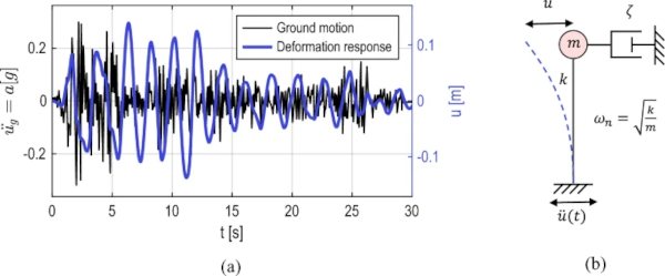
Most earthquakes are caused by the displacement of the tectonic plates and the resulting shear brittle fractures and frictional slip along the plate margins. The released energy is propagated on all sides by so-called longitudinal waves (P waves) and shear waves (S waves) (Petersen and Werkle 2017). During an earthquake, mass inertia forces act on the structures due to ground shaking. A ground motion of the Imperial Valley earthquake of May 18, 1940, recorded in north–south direction at a site in El Centro, California, is shown in black in Fig. 1a. The calculation of the response of the motion of a linear single-degree-of-freedom (SDF) system, as schematically illustrated in Fig. 1b, can be carried out according to (1) For a given ground motion u¨g(t), the deformation response u depends only on the frequency ωn, and its damping ratio ζ. The natural frequency ωn of an SDF depends only on the mass m and stiffness k of the system for small damping values. Both parameters, ωn and ζ are specific to each building and are influenced, for example, by the selected type of construction, the design, and the building materials utilized. The exemplary deformation of a SDF-system with a damping ratio ζ of 5% and a frequency ωn of 0.5 Hz is displayed in Fig. 1a in blue (Chopra 2012).

With: ωn = Natural frequency,ζ = Damping ratio, u = Displacement of the system, u˙ = Velocity of the system, u¨ = Acceleration of the system.

1.3 Structural design for buildings under seismic loads in building codes

This section provides a basic overview of the principles of structural design under seismic loads. Therefore, major variations between the different national standards exist, as the risk for seismic events varies highly in different regions. According to (Bachmann 1995) three basic properties in the seismic design are significant:

• The stiffness
• The load-bearing resistance
• The ductility

By increasing the stiffness against horizontal loads, displacements and floor shifts are decreased. Consequently, damage to non-structural parts like partition walls or facades can be minimized, which is particularly important for relatively weak earthquakes. To minimize plastic deformations in case of an earthquake, the load-bearing resistance has to be increased. Ductility or plastic deformation capacity describes the amount of energy that a building can absorb or dissipate during an earthquake. A certain amount of ductility is required to prevent a structure from collapsing during a design earthquake. These properties are embedded in the design-principals of the standards for the design of structures against earthquakes and have to be considered.

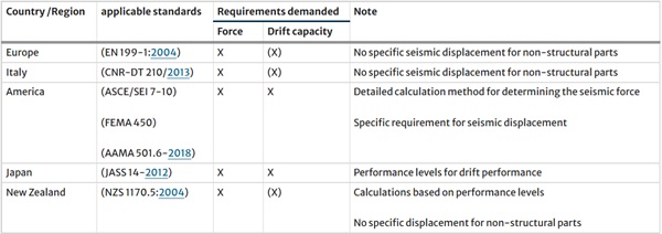
A good summary of the regulations worldwide can be found in (Scavino 2014). For Europe the Eurocode 8 (EN 1998-1:2004) defines the standard for the design against earthquakes, whereby country-specific regulations are regulated in the national annexes. Other important countries with high seismic activity are America ((FEMA 450, ASCE/SEI 7-10), Australia (AS 1170.4), New Zealand (NZS 1170.5), China (GB 5001-2001), India (IS 1893, IS 13935) or Japan (JASS14). For the design of structural components, the standards offer different methods for the calculation. On the basis of the EC 8 (EN 1998-1:2004), the following calculation methods are available for the verification of seismic safety:

• Lateral force method of analysis
• Modal response spectrum analysis
• Non-linear static (pushover) analysis
• Non-linear time history (dynamic) analysis

These methods differ highly in their complexity. In the design of new buildings, the first two methods are usually used in practice. Both methods have in common that the load due to the earthquake is applied to the buildings by means of equivalent static loads. Therefore, the calculation can be executed with similar tools as the static design, and less dynamic effects have to be taken into account. An introduction to the seismic design of steel structures is given in (Landolfo 2015).

1.4 Structural-Glazing-facade-systems under seismic load

The earthquake load on facade systems has been the subject of research for several decades. A comprehensive overview of seismic loading and experimental evaluation of non-structural curtain walls in buildings is given in (Huang et al. 2017).

For the design of glazed curtain wall facades, the building codes provide some limited guidelines. The most important regulations can be taken from (Galli 2010–2011; Memari 2013; Scavino 2014; Nardini and Doebbel 2015, 2016, 2020; Momeni and Bedon 2024) and will not be repeated in detail. In (Bedon et al. 2019), it is mentioned, that a so called behavior factor q = 1 is generally used for glass verifications. The behavior factor q is used with the lateral force method to reduce the elastic acceleration response spectrum to a so-called “design spectrum”. The capacity of structures to dissipate energy through plastic deformations is therefore taken into account, so the seismic design force is adapted in relation to a linear elastic response. Earlier versions of the Italian NTC standard suggest a q-factor of up to 2, but this is removed in the current document.

In general, the international standards define two main requirements to calculate the behavior of non-structural components:

• Transfer of a seismic-induced equivalent force due to the mass of the component
• Accommodation of deformation due to seismic inter-story drift of the main-structure

The calculation procedure in detail differs for all guidelines. For some of the most important regions with seismic activity, the standards for the regulation of the design of non-structural components are summarized in Table 1. In addition, the respective special features related to the requirements demanded are mentioned.

Table 1 Comparison of the most important regulations for glass-and facade structures under seismic loads in international standards - Full size table

One interesting subject worth mentioning is the concept of performance classes used in different guidelines. Here, the performance of a component after the occurrence of an earthquake is defined. This leads to economical and efficient dimensioning. For earthquakes with a small impact but a higher probability of occurrence, there should be no loss in performance, and the service state should be maintained. On the other hand, for the biggest earthquakes with a very rare occurrence, the goal is to reduce hazards through non-structural parts.

When concerning bonded facade structures, most studies deal with the failure of the glass in these facade-systems. Based on full-scale mockup tests, analytical and numerical models were developed to predict the failure and deformation behavior of SG-facade-systems. (King and Lim 1991; King and Thurston 1992; Thurston and King 1992) published the first investigations containing information on the behavior of SG-facade-systems. In (Zarghamee et al. 1996), the analyzed SG-construction was attached to the main structure by an adapted sub-frame to accommodate the movement from the building. With this design, the facade could withstand a seismic drift ratio of 1/50 without glass or adhesive failure in a mock-up test (Behr 1998). Studies that focus more on the structural behavior and performance are examined for two-sided SG facades in (Memari et al. 2006b; Memari et al. 2012b) and for four-sided constructions in (Broker et al. 2011). The complexity of the test facility increased for the four-sided curtain wall.

 Compared to the annealed monolithic specimen tested in (Memari et al. 2006a), the two-sided SG-facades (Memari et al. 2006b) show a 100% higher drift capacity (Behr 2009). Further tests on mock ups of unitized facade panels are provided by (Galli 2010–2011). Here inter-story drifts of H/300, H/200, and H/100 were imposed in accordance with the performance levels in (JASS 14-2012). A more in depth analysis of the deformation in the SG joint was carried out in (Nardini and Doebbel 2015, 2020). (Bianchi et al. 2022) deals with the serviceability and ultimate seismic performance of unitized curtain walls. In addition to the calibration of numerical modeling, and the study of the damage mechanism, the influence of facade details on the seismic behavior is investigated. An improved method for numerical modeling of curtain walls is presented in (Nuñez Enriquez 2022). (Hayez et al. 2023) provides an overview of the most recent test program for large component tests as well as of different FE and experimental-based preliminary tests. A complete evaluation of the tests has not yet been presented.

Some minor studies examine in detail the behavior of the SG joint under and after cyclic loading to simulate the specific fatiguing characteristics of earthquake loads. In (Zarghamee et al. 1996) a cyclic fatigue test was performed, in which the sealant was loaded between 0.069 MPa and 0.138 MPa for 50 cycles. Another cyclical testing method is proposed in (Broker et al. 2011; Memari et al. 2012a). Here, tensile and shear samples of a one- and a two-component SG-adhesive were investigated according to (ASTM C1184-18e1) criteria. The cyclic stress level was chosen based on (Zarghamee et al. 1996) with 0.345 MPa, to which the samples were loaded and relaxed for four cycles. On the final cycle, the samples were pulled until failure. No relevant influence on the ultimate stress could be determined for both adhesive types, according to the authors. 

The visible difference in the load path is the characteristic “Mullins” effect (Mullins 1948) of SG-adhesives, which was investigated in numerous studies (Palmieri et al. 2009; Schaaf et al. 2021). (Nardini and Doebbel 2016, 2020) used the Hockman cycle (ASTM C719-93) to simulate the effect of cyclic loading on the adhesive after an earthquake event. This method consists of cyclic testing to a defined elongation rate at room, as well as high and low temperatures after immersion in water for 7 days. The elongation rate is defined as 12.5% and 25% to investigate the performance of the adhesive on two levels. As a result, a clear reduction in final strength can be shown for the specimen loaded repeatedly to 25% elongation. In (Zarghamee et al. 1996) it is noted that the Hockman cycle(ASTM C719-93) with a total duration of about 400 h may not be sufficient for testing the degradation through seismic motion.

In summary, it is shown that cyclic loading of SG adhesives can have an influence on both the ultimate strength and the stiffness.

2 Methodology

2.1 Motivation and problem statement

As described in the introduction of this paper, there is currently no reliable scientific knowledge available to describe the structural performance of SG adhesives in glass and facade construction during and after seismic events. In particular, the systematic description of the effects of cyclic-dynamic loading on material properties cannot be done on the basis of the existing database.

The current knowledge of the material behavior under cyclic loading is not sufficient for the safe and economical design of structural SG connections against seismic loading, especially for increasingly larger and more complex facades or all-glass structures. The aim of this publication is therefore to extend the basic understanding of the behavior of the SG connections under seismic loading. As previously outlined in Sect. 1, earthquake loading typically comprises a series of randomly consecutive load cycles with varying load levels. This repetitive loading can be categorized within the domain of low-cycle fatigue loading, which is typically defined within the range of up to 10⁴ load cycles. Therefore, the relevant influencing parameters are identified and narrowed down to areas of practical relevance. The results will be used as a basis for proposing the engineering dimensioning of SG joints for seismic loads.

The following specific issues are addressed in this publication:

• What load-bearing behavior do SG adhesives exhibit under low-cycle fatigue loading?
• What are the parameters that influence the low-cycle fatigue performance of SG joints and can they be narrowed down?
• What influences can be determined for the load-bearing behavior under low-cycle fatigue?

2.2 Scope and outline

The following methodology is chosen to answer the scientific questions:

The first step will be an assessment of the stress due to seismic loading on SG adhesives in structures used in glass and facade construction. In the first step, typical glass and facade structures will be selected and the load specific differences due to different constructions will be analyzed. This is followed by a more detailed investigation of the seismic loading on SG adhesives. For this purpose, a structural model of a multi-storey building is created as a beam-column or skeleton structure. To evaluate the stresses in the SG joints, a sample bonded facade element is added to the model. The foundation of the structure is loaded by the ground acceleration of an exemplary earthquake and the resulting stress on the bonded joint is evaluated. To analyze the relevant load frequencies during the earthquake, the loads are determined by evaluating response spectra generated from several historical earthquakes. Other parameters influencing performance under cyclic loading are identified and narrowed down from a literature review. Based on this detailed assessment of the seismic loading characteristics, the experimental test matrix is defined. The specimen manufacturing and the experimental test setup are described in detail, as both have a significant influence on the variability of the experimental test results. In addition to the cyclic tests under low-cycle fatigue loading, static reference tests are performed. The quasi-static reference performance section describes the typical shear performance of SG adhesives. In particular, a method for evaluating the cyclic strength based on these statistically verified material parameters is presented.

In order to obtain an initial overview of the structural behavior under seismic loading, tests are carried out under cyclic single-stage loading at a high load level. With the help of this type of loading, a systematic analysis of the relevant influencing parameters and thus an assessment of the randomly occurring earthquake load is possible for the first time.

First, the basic load-bearing behavior is analyzed on the basis of the hysteresis that appears in the stress–strain diagram, and the effects of the type of load application are highlighted. In the following section, the typical hysteresis presentation generated from the test data is converted into a cyclic stress–strain curve (CSSC) to analyze the previously selected influencing parameters. This provides a clearer representation of the cyclic load-bearing behavior under cyclic loading. Using these CSSCs, the effects of the selected influencing parameters on the cyclic performance are evaluated. Finally, an outlook on possible future problems is given.

3 Stress assessment

3.1 General

There are a large number of influencing parameters when investigating cyclically stressed adhesive bonds, particularly due to the viscoelastic load bearing characteristics. In the following section, the most relevant parameters for glass and facade structures under seismic loading are selected and narrowed down. The influencing parameters selected in this section are then analyzed in the experimental investigations.

3.2 Relevant glass- and facade structures

The continued development of SG as a construction method, and the associated increase in confidence, has made it possible to design and construct increasingly complex structures. In addition to classic facade constructions, such as the example shown in Fig. 2a, it is now possible to design and construct self-supporting all-glass structures, as shown in Fig. 2b.

In both types of construction, the adhesive joint is usually designed as a linear joint. In facade constructions, SG adhesives are used to bond the glazing to the substructure. The joint is subject to normal loads in the tension–compression direction due to the effect of wind and in the shear direction due to the different coefficients of thermal expansion of the various materials. In all-glass constructions, there is an additional shear load in the joint due to the stiffening effect of the connected glass elements.

3.3 Analysis of the seismic load

3.3.1 Development of a simulation model

When analyzing the loads on SG joints in glass and facade constructions, a combined load of tension and shear loads on the joint is obtained. Based on (ETAG 002-1) and various scientific papers such as (Hagl 2006, Schuler et al. 2017, Bues 2021), a separate analysis of the two load directions, tension and shear, is performed in this publication.

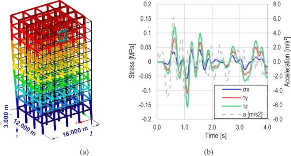
To analyze the load on the SG joint, an engineering calculation model is created using the Dlubal FE software ‘RFEM 5’ according to (Murty et al. 2012; Bhuskade and Sagane 2017). The beam-column structure of the concrete structure with a regular grid of 4 m and a floor height of 3 m is simulated as a framework. The beam cross-section is 300 × 400 mm² and the column cross-section is 800 × 800 mm². An overview of the framework model with global dimensions is shown in Fig. 3a. To account for the dead load of the structure, the building is loaded floor by floor with a surface load of 4.0 kN/m² in addition to the dead load of the structure. This self-weight is used as a mass in the dynamic calculation.

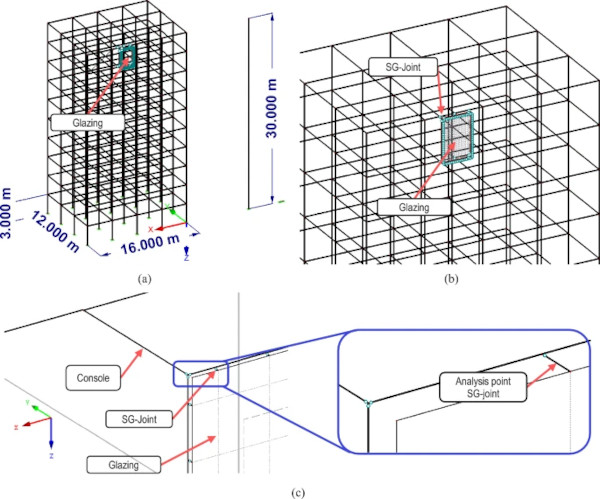
To perform an initial basic load analysis of the SG joint in a facade glazing, an exemplary glazing is placed in a field of the concrete structure, as shown in Fig. 3b. In addition to the position of the glass element on the top floor, a glass element on the first floor was also examined in preliminary studies, and no relevant differences in load height were found. The load curves over time also show a general agreement. For a clearer presentation of the results, only the top floor pane is analyzed in this publication. This is based on the assumption that the additional glazing does not significantly affect the stiffness and therefore the natural period of the structure and that the representation of one glazing unit is sufficient.

The SG bond is modeled according to (Fachverband Konstruktiver Glasbau e.V. 21.09.21, Müller et al. 2023b) with dummy rod between the glazing and the mullion. The dummy rods are spaced 100 mm apart and have a rectangular cross-section of 12 × 100 mm² and a length of 12 mm to simulate the assumed dimensions of the 12 × 12 mm² SG joint. The calculation is performed with linear elastic material behavior and an Young’s modulus of 4 MPa and a Shear-modulus of 0.67 MPa. The load on the bonded joint is evaluated at the center of the dummy rod. The modeling of the bonded joint, including a detail of the dummy rod, is shown in Fig. 3c. An overview of the main components of the FE model including material properties is given in Table 2.

Table 2 Overview of FE model components including material properties - Full size table

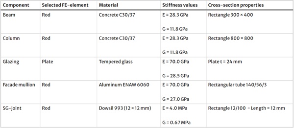
Based on this calculation model, the dynamic properties of the structure were determined, taking into account the dead load of the structure. This results in a maximum natural period of 1,057 s, shown in Fig. 4a, which is a realistic value for a multi-storey structure according to (Chopra 2012).

3.3.2 Determination of load direction

For the SG joint load analysis, the entire building structure is loaded with a dynamic load case on all supported columns. The “Loma Prieta” accelerogram from the “Corralitos—Eureka Canyon Road” measuring station of 1989-10-17, 17:04, which is stored in the software, is used for this purpose. A section of the acceleration history is shown in Fig. 4b in gray.

The highest stresses were determined in the dummy rods in the corners of the glazing using an SRSS result envelope from a response spectrum calculation. The dummy rod in the upper-left corner, as shown in Fig. 3c, is therefore used to analyze the load on the bonded joint over time. To do this, the internal forces over the cross-sectional area are converted to stresses and plotted in Fig. 4b. Looking at the stress distribution over time, the load is present in a series of a few, randomly consecutive cycles acting in all load directions. This load pattern is typical of seismic loading. Other dummy rods selected as examples also show the typical random shear-dominated load pattern.

With a maximum value of the shear stress τZ of about − 0.15 MPa, the load level is within the application limits of the calculation method from (Fachverband Konstruktiver Glasbau e.V. 21.09.21). It should be noted, however, that the load level is to be regarded as purely exemplary, since almost any change is possible by adjusting the adhesive joint properties or the building geometry. However, the method seems to be sufficient to provide a first overview of the stresses induced by a seismic event, in particular, the relationships between the different stress components. The diagram in Fig. 4b shows that the tensile load is exceeded by the shear load by approximately 87% in the y-direction and by more than 170% in the z-direction. Based on this simplified view, it can be seen that during seismic actions, the bonded joints experience the highest load in the shear direction parallel to the joint axis. Therefore, only the shear-stressed bonded joint is considered in the following publication.

3.4 Influencing parameters for cyclic testing of adhesives

When analyzing the performance of SG joints under cyclic seismic loading, there is a virtually infinite number of influencing parameters and parameter combinations. These must be determined in the first step and then narrowed down based on engineering estimates. A good overview of the decisive parameters influencing standard high-cycle fatigue tests can be found in the “LebKleb” research project (Ciupack et al. 2018). Cyclic loading tests with constant amplitudes were performed on standard composite specimens and component-like specimens. Both 2-part polyurethane and acrylate adhesives were used. The following parameters were investigated in the standard cyclic tests:

• Load level
• Mean stress effect
• Temperature
• Test frequency

In addition, the following other parameters may be present when investigating the effects of earthquakes on SG adhesives:

• Type of load applied by the structure
• Load direction
• Joint geometry

Based on engineering considerations, the influencing parameters to be investigated are narrowed down below.

3.4.1 Mean stress effect

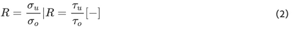
The mean stress effect can be characterized by the stress ratio R as shown in (2). The typical cases for the stress ratio can be named as cyclic alternating loading (R = − 1) and cyclic threshold loading (R = 0). Two cycles for these stress ratios are shown in Fig. 5a.

With: σu/τu= Minimum tensile/shear stress

σo/τo= Maximum tensile/shear stress.

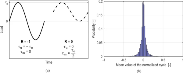
To obtain an initial overview of the stress ratio R in seismic loading, 153 ground motion histories from the (Ancheta et al. 2013) database were analyzed. The first step was to normalize the load-time histories to make them comparable. A rainflow count of these load histories was then carried out to determine the mean value of the individual cycles in addition to the stress range. In order to focus the evaluation on the damage-relevant cycles, only the cycles with a stress level of at least 20% of the maximum value are considered. A total of 3954 cycles were analyzed and are shown in the histogram in Fig. 5. With the histogram peak at the mean value of 0, it can be demonstrated that the alternating load with an R ratio of -1 best represents the earthquake load.

Based on these evaluations, the experimental studies will focus on the analysis of load cycles with a stress ratio R of -1. In addition, based on the fatigue cycles used in (Zarghamee et al. 1996; Memari et al. 2004, Broker et al. 2011)), an R ratio of 0 is also analyzed to compare with the results from the literature.

3.4.2 Temperature

As shown in (Schuler et al. 2017; Schuler et al. 2023), temperature has only a minor influence on silicone adhesives compared to other adhesive types. Therefore, this parameter will not be considered in further investigations.

3.4.3 Test frequency

Due to the different vibration durations of the building structures, the load on the bonded joint occurs at different frequencies, which is why this parameter should be investigated. The test frequency can be approximated by using the response spectra of historical earthquakes.

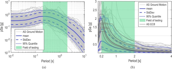
For this purpose, the response spectra of a total of 153 load-time histories of past earthquakes were used to determine the relevant range of load frequencies during earthquake loading. The response spectra were calculated using the (Ancheta et al. 2013) database and are shown in Fig. 6a. In addition to the mean, the standard deviation and the 0.05 and 0.95 quantile curves are shown for clarity. For better reference, all standardized elastic spectra from (EN 1998-1:2004) were calculated and are additionally shown in Fig. 6b. In general, there is a good correlation between the real response spectra and the standardized spectra from EC8. This is a good indicator that a reasonable selection of load-time histories has been made and that the existing variance in the load is well represented.

It can be seen that from an oscillation period of just under 1 s, the load starts to decrease from the plateau region. In the case of the 95% quantile curve at 2 s, the load is only about 25% of the maximum acceleration. The load is highest at a period of 0.2 to 2 s or a frequency range of 0.5 to 5 Hz, so this range is analyzed in more detail in this publication.

3.4.4 Type of load application

In order to analyze the type of load action, a distinction must be made between the two types of construction mentioned in Sect. 3.2 . In the case of a classical facade construction, the glazing can be described as a secondary component. In the event of an earthquake, the foundation of the primary structure is first excited and then the bonded joint is deformed and loaded by an applied forced deformation. In all-glass structures, the glass, and therefore the adhesive bond, is the primary structure of the building. In the event of an earthquake, the glazing, including the bonded joints, is directly excited by seismic waves.

In order to reflect this different behavior in the experimental investigations, the following types of control are distinguished:

• Secondary structure: Displacement-controlled test execution
• Primary structure: Force-controlled test execution

3.4.5 Load direction

As shown in Sect. 3.3 , SG joints are subjected to both shear and tension loads during a seismic event. As the load level in the shear direction is significantly higher than in the tensile direction, only the shear behavior is considered in this publication.

3.4.6 Joint geometry

As part of the approval process, a joint cross-section of 12 × 12 mm² is usually examined on the basis of (ETAG 002-1). In order to investigate the influence of different joint geometries, an adhesive joint of 8 × 24 mm² is also examined, which represents the limit value of joint width to joint heigt hc/e≤3, up to which the application of (Fachverband Konstruktiver Glasbau e.V. 21.09.21, ETAG 002-1) is possible.

4 Experimental investigations

4.1 specimen manufacturing

4.1.1 Joint dimensions, material and preparation

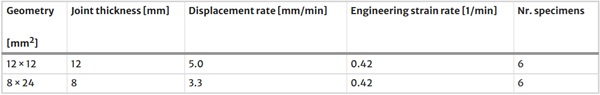
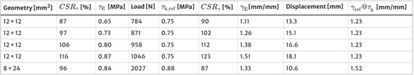
The general specimen manufacturing process for the specimens in this publication is based on (Müller et al. 2023b). The principal shape of the modified H-specimen is based on the specifications in (ETAG 002-1) and was developed by (Schuler et al. 2017; Bues et al. 2019; Bues 2021). In addition to the standard geometry of 12 × 12 mm², a joint geometry of 8 × 24 mm² is investigated, which represents the limit value he/e ≤3. to apply the calculation method according to (ETAG 002-1) or the spring model according to (Fachverband Konstruktiver Glasbau e.V. 21.09.21) without further stiffness investigations. The width of the joint hc slightly exceeds the limit of hc≤20mm according to (ETAG 002-1). The length l of the modified H-specimen is increased from 50 to 100 mm compared to the ETAG H-specimen geometry to more accurately reproduce the behavior of a continuous joint (Schuler et al. 2017; Bues et al. 2019). The geometries studied are summarized in Table 3.

Table 3 Joint geometries of the investigated modified H-specimens - Full size table

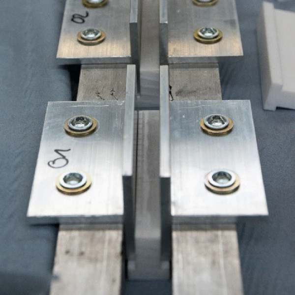
Two T-profiles (T 50 × 50 x 5 mm3) made of natural extruded aluminum (EN AW 6060 T66) were used as a support profile to provide a rigid load path to the adhesive for the modified H-specimen used in these investigations. The rigid connection between the specimen and the testing machine ensures that the results are not influenced by deformation of the test fixture or slippage, particularly in the early part of the test. Prior to bonding, the aluminum was cleaned and wipe-degreased with isopropanol. After cleaning, the adhesive manufacturer’s recommended primer was used prior to adhesive application.

Since the cohesive fracture pattern required by (ETAG 002-1) could be obtained in all tests in this publication, it is assumed that the substrate surface has no relevant influence on the results of the tests shown here.

In addition, it should be noted that the surface of the substrates can have a significant effect when analyzing, for example, the artificial aging behavior of SG adhesives or when planning real constructions. Only substrates that meet the manufacturer’s specifications should be used here. The approach proposed here seems reasonable in the interest of performing economic load tests. For further testing, the fracture pattern must continue to be monitored consistently to avoid influences. All specimens tested for this publication were manufactured with natural aluminum surfaces.

4.1.2 Manufacturing

The specimens were manufactured under controlled laboratory conditions using a two-part silicone DOWSIL™ 993 commonly used in the facade industry for structural glazing systems. The adhesive was processed in an industry standard mixing and dispensing system. Production took place at the company seele in Gersthofen, Germany. To minimize variations due to different batches of adhesive, all specimens tested in this publication were manufactured on the same day using the same adhesive.

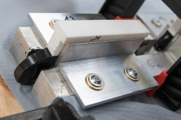
Prior to the bonding process, the T-profiles were perpendicular aligned and secured to mounting profiles. Polytetrafluoroethylene (PTFE) plastic spacers were placed under the T-profiles to achieve precise cross-sectional dimensions, as shown in Fig. 7. The joints were filled with adhesive from the top from one side to the other. After filling, the second plastic spacer was pushed into the gap, allowing excess adhesive and air to escape on both sides. The two mounting profiles were clamped together with two clamps (Fig. 8) to secure the plastic spacers and to obtain the exact height of the joint. After curing for at least 2 days, the plastic spacers were removed and the excess adhesive was cut off with a sharp knife. The end of the finished specimen after cutting off the excess adhesive is shown in Fig. 9 for the two joint geometries.

All specimens were cured with the method “40 °C” according to (Müller et al. 2023b). Therefore, after manufacturing, the specimens were stored at room temperature for 7 days and then at 40 °C for 13 days in a heating chamber. After tempering, the specimens were post-cured at RT for at least 1 day to recondition them.

Prior to testing, the actual dimensions of the joint were measured using a digital caliper. All evaluations in this publication are based on actual dimensions to avoid overestimating load carrying capacity of the adhesive.

4.2 Testing

4.2.1 Quasi-static reference tests

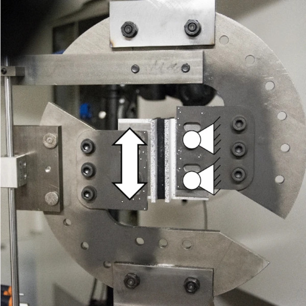
To determine the quasi-static reference load-bearing capacity, 6 modified H specimen per joint geometry were tested. Based on these tests, statistically validated parameters such as the characteristic failure stress τk or failure strain γk can be calculated. The specimens were tested under a global shear load, which is related to a load acting parallel to the joint. The tests were performed in a 100 kN universal testing machine, “Instron 5982”, with an interposed 10 kN load cell under displacement control. The displacement rate was selected according to (ETAG 002-1) with 5.0 mm/min for the joint with a height of 12 mm. The displacement rate of 3.3 mm/min was chosen to maintain the engineering strain rate for the 8 mm joint. Strain and load rates for the joint dimensions tested are listed in Table 4. The specimens were bolted into a rigid test fixture made of 10 mm thick steel. Displacement was measured by deformation of the crosshead travel of the testing machine. The test setup is similar to the cyclic tests shown in Fig. 10.

Table 4 Loading and strain rates - Full size table

4.2.2 Low-cycle fatigue investigations

A “Schenck” servo-hydraulic test frame with a PL10K longitudinal cylinder installed was used to perform the cyclic tests. The load cell used in the test frame is a 1720ACK load cell manufactured by “interfaceforce” with a measuring range of 10 kN in tension and compression. The test system is controlled by an EU3000 digital measurement and control system and the associated TestControl software. The manufacturer is “inova”. Depending on the tests to be performed, the test is controlled by force or displacement control with peak value control activated. The required PID values of the controller were determined in preliminary tests for the different test parameters. A compromise had to be found between the stability of the test sequence, the accuracy of the load level and the constancy of the load level. Especially for the force-controlled tests, the constancy of the load level was prioritized so that the actual load level was slightly below the planned level. The subsequent determination of the actual load level ensured correct test evaluation. The test setup for the cyclic test is shown in Fig. 10.

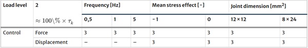
In order to provide the best possible overview of the cyclic behavior, the most relevant parameters from Sect. 3.4 are examined in this publication. Due to the large number of influences, a fully parametric combination of all influences does not seem to be appropriate. To determine the influence of the type of load or test control and the load level, these two parameters are combined in a first step. The load levels for the cyclic tests are based on the characteristic fracture shear stress τk based on quasi-static reference tests. The reference load bearing behavior will be evaluated in Sect. 5. These tests are performed at a frequency of 1 Hz, a stress ratio of -1, and for joint dimensions of 12 × 12 mm². The resulting test matrix is shown in Table 5. Based on this, the parameters that have not yet been varied are determined in a second step at a load level of 100%, resulting in the test matrix in Table 6. Due to the number of specimens available, only force-controlled tests could be performed for frequency analysis.

Table 5 Test matrix on the influence of load level and test control - Full size table

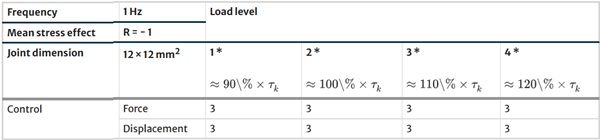
Table 6 Test matrix on the influence of frequency, stress ratio, and joint dimensions - Full size table

5 Quasi-static reference load bearing behavior

5.1 General load bearing behavior

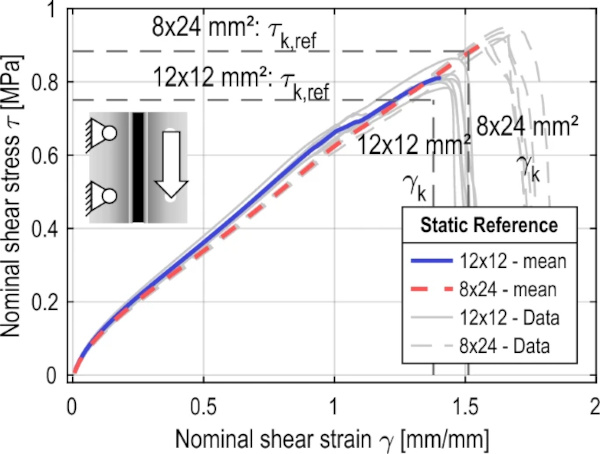
The structural behavior of SG joints has been extensively studied in (Schuler et al. 2017; Bues et al. 2019; Bues 2021; Schuler et al. 2023). The stiffness under shear load depends primarily on the deformation capacity of the adhesive, which can be described by the shear modulus G. The specimen type and the joint geometry have no significant influence on the deformation behavior of the bond. With respect to the maximum load-bearing capacity, it was found that different levels of strength are obtained depending on the specimen type and joint geometry.

These results can be confirmed by the reference tests performed here. The stress–strain curves of the two reference series are shown in the diagram in Fig. 11. The 6 individual curves for each joint geometry are shown in gray and can be distinguished by their line type. For a better comparison of the load-bearing behavior, an average curve was calculated from all the curves up to failure of the first specimen, which is colored according to the joint geometry. In general, the two series behave very similarly. A non-linear decrease in stiffness can be observed up to a stress of about 0.2 MPa. Beyond that, the curves show an almost linear progression. Failure occurs much earlier in the series with the 12 × 12 mm² joint geometry.

5.2 Statistical evaluation and definition of load levels

5.2.1 Statistical evaluation

To determine the load levels for the cyclic tests and to account for the effects of specimen charge, characteristic parameters for specimen strength and stiffness were determined from the stress–strain curves and statistically evaluated, as investigated in (Müller et al. 2023b).

According to (ETAG 002-1), the initial mechanical strength is represented as the average ultimate failure shear stress τult of all specimens. For a general statistical interpretation, the characteristic breaking stress τk, defined as the 75% confidence interval of the 95% quantile of the test results, can be calculated using Eq. (3). The determination of the fractile factor k3 requires the application of the non-central Student’s t-distribution with a non-centrality parameter δ (Beech and Owen 1962; Loch 2014). For practical use, values for the k₃ factors are given in (ETAG 002-1, ISO 16269-6:2014-01). For the purpose of this publication, the calculation of the characteristic failure stress τk has been performed according to (ETAG 002-1). This ensures the best possible comparability with the manufacturer’s value σk,ETA.

With: τk= the characteristic breaking stress (75% confidence that 95% of the test results will be higher than this value [MPa]

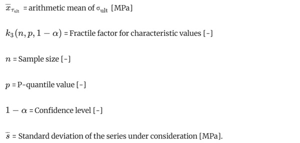
The elongation at fracture γult of the specimens is determined to describe the deformability, contrary to the determination of the secant modulus K₁₂.₅ at 12.5% elongation proposed in (ETAG 002-12). The (ISO 527-1:2019) describes the elongation at fracture as the elongation value, before the stress decreases to less than or equal to 10% of the tensile strength. This definition can have the disadvantage when analyzing the modified H specimens, especially under shear loading, that there is often some residual capacity even after a significant reduction in stress, so that the criterion of (ISO 527-1:2019) is not met. This leads to long test times and high scatter. To counteract this, the fracture strain γult is defined in this publication as the slip of the specimens at the moment of maximum fracture stress τult. The characteristic fracture strain γk is also determined for the fracture slip γult based on Eq. (3).

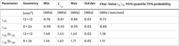
The results are presented in Table 7. It can be seen that both the fracture stress and the fracture slip of the 12 × 12 mm² specimen are lower than those of the 8 × 24 mm² specimen. Both the series and the characteristic values have very small standard deviations, resulting in a relatively small reduction in the determination of the characteristic values.

Table 7 Summarized statistical evaluation - Full size table

5.2.2 Evaluation of the load levels

The load levels for the cyclic tests were defined on the basis of characteristic values from extensive preliminary tests. As shown in (Müller et al. 2023a, 2023b), an influence of the specimen manufacturing must be assumed. In addition, as described in Sect. 4.2.2, the combination of high loading rates, large deformations, and nonlinear material behavior poses a great challenge to test execution and control. In the force-controlled tests, the PID control parameters could only be set to achieve a constant load level while maintaining a stable test sequence. The load level deviated slightly from the controlled value. To determine the real acting stress τE, the maximum load of each cycle was determined from the test data as part of the test evaluation, and τE was then calculated as the average of all the maxima.

In order to minimize the influence of the production series and the joint geometry and to allow a comparison of the types of test control, the cyclic stress ratio (CSR) was determined in the further evaluation. The evaluation of cyclic laboratory tests via the definition of the CSR has been proposed in (Seed et al. 1975; Green and Terri 2005), particular for the cyclic liquefaction evaluations of soil under seismic loading. In this publication, the real applied stress τE was related to the characteristic failure stress τk of the reference tests of the specimen series for the force-controlled tests. The CSRτ for the force-controlled tests is therefore defined as the ratio between the applied stress τE and the characteristic failure stress τk, as in Eq. (4). The CSRγ for the displacement-controlled tests is determined similarly to Eq. (5). The effective slip γE is determined from the maxima of the test data in the same way as for force control. The basis is the slip γref@τk at the location of the characteristic fracture stress τk from the mean curves in Fig. 11 and Table 7.

Evaluation of the CSR allows comparability between the two types of loading. A summary of the stress levels is given in Table 8.

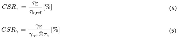
Table 8 Load levels for the cyclic tests - Full size table

6 Low-cycle fatigue performance

6.1 Fundamental low-cycle fatigue behavior

All cyclic tests were performed as displacement or force-controlled tests, depending on the test control selected. A sinusoidal load curve was selected as the shape of the load-time curve, as shown in Fig. 12as an example. The raw and unfiltered signal from the testing machine was smoothed for all samples using MATLAB ® software to ensure better post-processing of the data. A quadratic regression smoothing method with a width of 0.04 s was chosen. On the one hand, the noise of the data could be filtered very well, on the other hand, no relevant influence on the measured data could be detected.

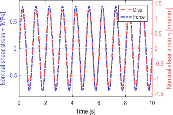
With the selected control parameters of the machine, a sinusoidal load curve with constant maximum load could be achieved for both control types despite the highly nonlinear material behavior of the SG silicone, as can be seen in Fig. 12.

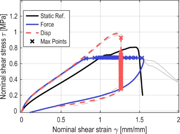
To better analyze the load-bearing behavior, the data from the two series of tests in Fig. 12 are plotted on a stress–strain diagram. The resulting hysteresis is shown in Fig. 13. Figure 13a gives an overview of the entire stress and strain range. Figure 13b shows only the positive range of the test to facilitate the analysis of the two curves. In addition to the two cyclic tests, a sample stress–strain curve from an explicit quasi-static reference test is shown for comparison. A deliberate decision was made not to plot the average curves from Fig. 11 because they do not show the failure of the sample.

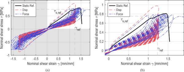
The analysis of the first load path shows very similar behavior for both control types. Compared to the static reference curve, the bearing behavior of the cyclic test is slightly stiffer, which can be explained by the significantly higher loading rate, as confirmed by (Bues 2021). For the displacement-controlled test, this stiffer bearing behavior results in a maximum stress that is relevant above the failure stress τult of the quasi-static test. Therefore, it can be assumed that the specimen is significantly overloaded in the first cycle. This high load is not seen in the force-controlled test.

Looking at the shape of the first hysteresis of both tests, it has a significantly larger area compared to the subsequent ones. This phenomenon can be partially explained by the typical Mullins effect (Mullins 1948). Also typical is the significantly stiffer load-bearing behavior at the beginning of the first cycle and the clear difference in stiffness between the first and subsequent cycles.

The stiffness of the specimen decreases steadily during the test, with differences in the curves for the two control types. In the displacement -controlled test, the allowable stress of the specimen decreases during the test and relaxation occurs. In contrast, in the force-controlled test, the stress remains at a constant level, the strain increases during the test, and a plateau region is formed. This behavior can be compared to creep (Gent 2012) or defined as retardation (Schröder 2018).

Significant differences can also be observed in the failure behavior of the specimens. In the last cycle of the force-controlled test, the applied load can no longer be applied to the specimen, resulting in an increase in deformation and finally a sudden failure of the specimen. This failure behavior can be observed in the diagram in Fig. 13a at a stress of approximately − 0.75 MPa and a strain of -1.8 mm/mm. In contrast to this sudden failure, the stress that can be absorbed by the specimen continues to decrease in the displacement-controlled test. However, a complete or sudden failure of the specimen cannot be observed. Without additional termination criteria, the test would continue virtually indefinitely. For this reason, it is pragmatic to define the end of the test based on a predetermined percentage change in stress during the test. For the displacement -controlled test results in this publication, a drop in the absolute stress of the current cycle to less than 30% of the maximum stress in the first load cycle has been defined. It should be noted, however, that the method used here to define the cutoff limits is one that is commonly used in cyclic testing. The limit for the final cutoff was freely chosen.

Alternatively, many other criteria can be defined to determine the end of the test. The influence of alternative termination methods and limits could be investigated in future publications and is beyond the scope of this report. However, this relationship should be considered, especially when interpreting the test results.

6.2 Cyclic stress–strain curves

6.2.1 Overview

For a clearer representation and subsequent analysis of the load-bearing behavior under low-cycle fatigue loading, so-called cyclic stress–strain curves (CSSC) can be generated from the representation of the entire test sequence, as shown in Fig. 13 (Götz and Eulitz 2022). For this purpose, only the maximum points of the controlled signal are plotted and connected in the diagram after the first loading of the stress–strain diagram. This gives the CSSC in Fig. 14 from the hysteresis in Fig. 13b. In all of the following illustrations of the CSSC, the colored curves, including the maximum points, are representative curves of an exemplary test procedure. The gray curves show the remaining samples in the series with the same line type to illustrate the variance. Average curves are not shown for clarity and due to the small variance within the series.

6.2.2 Type of load application

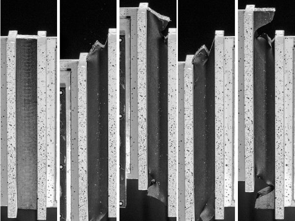
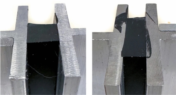
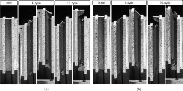
The different failure behavior resulting from the two types of test control and the differences in the first load cycle can also be determined from the CSSC. However, the information about the size of the area of each hysteresis is lost. The difference in failure behavior between the two types of test control can be well illustrated using the CSSC. The distance between the individual hysteresis maxima can be better visualized with the CSSC. It can be seen that the displacement-controlled test has a significantly larger distance or a larger drop in stiffness in the first cycle. To explain this difference, the crack propagation in the bonded joint is considered. For this purpose, Fig. 15 shows images of the bonded joint shortly after the maximum load at different test times. In the first load cycle, there is almost no damage to the specimen in the force-controlled test. In contrast, there is a clearly visible crack in the bonded joint of the displacement -controlled test. This means that the loss of stiffness in the force-controlled test is mainly due to the Mullins effect. In the displacement-controlled test, this is combined with a reduction in stiffness due to the clearly visible damage. After 10 cycles, a comparable level of damage is observed between the two specimens.

The behavior of the displacement-controlled test, which is comparable to a relaxation phenomenon, contrasts with the failure plateau that forms under force control. As mentioned earlier, this can be compared to a creep phenomenon and the CSSC is similar to the stress–strain curve of steel in the quasi-static tensile test. Looking at the scatter of the CSSC within the two series shown, there is very good agreement between the three individual curves. The small deviations indicate a high quality of the tests and a low level of unknown scatter within the test series. The clearer representation of the CSSC is preferred for the analysis of the following parameters.

6.2.3 Load level

The influence of the different load levels is shown in Fig. 16 for the two types of test control. A sample curve for each load level is shown in color, including the maximum points. The remaining curves of the same load level are shown with the same line type.

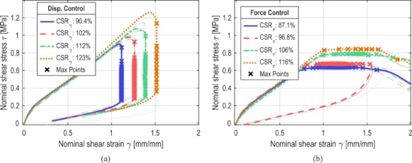
The CSSCs for both types of test control show very similar stiffness behavior. For the displacement-controlled tests shown in Fig. 16a, specimen failure occurs at each defined strain level. It is noticeable that the largest decrease in stiffness, as indicated by the distance between two maxima, occurs between the first and second cycles for all load levels. In addition to the already mentioned Mullins effect, this can also be explained by the considerable pre-damage of the specimen caused by the first overload. The distance between the individual maxima increases with increasing load level, indicating higher damage per cycle. It can therefore be assumed that the number of tolerable load cycles decreases as the load level increases. The maximum of the last cycle also increases with the load level, which can be explained by the definition of the shutdown criterion.

In principle, very similar results were obtained for the force-controlled tests in Fig. 16b. What is noticeable here, however, is the much more uneven spacing between the four load levels that were equally selected in the original test design. A possible explanation for this can be found in the control technology of the testing machine. The requirements are very complex due to the high deformations, the high test speed combined with the non-linear material behavior of silicone and the simultaneous failure of the specimen. A compromise was made in the choice of control parameters in the preliminary tests to ensure stability of the test procedure and uniformity of loading over the course of the test. Using the evaluation method selected in Sect. 5.2.2, the actual load is determined from the test data and can be used for further evaluation. Therefore, the deviation from the design loading level determined here does not negatively affect further analyses.

Looking at the failure behavior of the specimens loaded in the force-controlled test, a plateau region can be seen at all load levels where the specimen gradually fails. Complete failure of all specimens occurs at a strain range of approximately 1.5 mm/mm. As with the displacement-controlled tests, the distance between the maxima increases with load level, indicating greater damage per cycle.

Again comparing the effect of test control over all load levels, it can be seen that there is a uniform spacing of the maxima after the first few cycles for both types of control. For the force-controlled tests, this uniform spacing increases toward the end of the test, resulting in a significantly faster and more sudden failure of the specimens. In the displacement-controlled tests, the spacing remains constant.

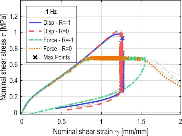
6.2.4 Test frequency

The effect of test speed or test frequency is shown in Fig. 17. The tests were performed under force control only. This shows a very similar load bearing behavior of the three series. Only the initial stiffness increases slightly with increasing test frequency due to the higher test speed. The test series with a frequency of 5 Hz shows a slightly slower final failure, which also starts at a shear strain of 1.5 mm/mm.

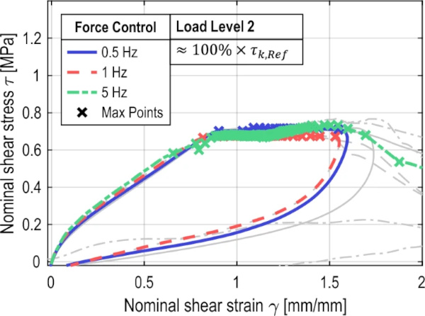
Overall, the distance between the maxima decreases as the test frequency increases, resulting in a higher number of load cycles that can be recorded.

6.2.5 Mean stress effect

The influence of the mean stress effect R is shown in Fig. 18. Both types of test control show similar load-bearing behavior in the short-term strength range. For the force control with an R ratio of 0, the distance between the maxima increases at a lower shear deformation of about 1.25 mm/mm. This may be associated with a slightly earlier onset of ultimate failure. A similar phenomenon can be seen in the displacement-controlled tests, where the distance between the maxima increases before the end of the test for the test with an R ratio of 0.

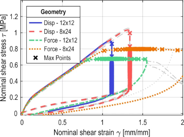
6.2.6 Joint dimension

The CSSCs of the test series used to analyze the influence of joint dimensions are shown in Fig. 19. Two series were compared under both force and displacement control, loaded as close as possible to the same CSR. The higher load on the series with the compact 8 × 24 mm² joint can be explained by the higher strength in the quasi-static tensile test from Sect. 5. The two joint geometries show very similar load bearing behavior under low cycle fatigue loading, regardless of the type of test control. These exemplary tests of the applicability of the results to alternative joint geometries do not indicate a fundamentally different behavior of the compact joint. Transferability of the results to joint geometries within the limits of (ETAG 002-1), and thus to full-scale components, appears to be possible in principle. This should be verified in further investigations.

7 Conclusion and future research

This paper presents investigations to improve the understanding of the material behavior of SG joints under low-cycle fatigue loading in shear. The first step was to perform out a stress assessment to identify and narrow down possible relevant influencing parameters. The relevant influencing parameters identified by the stress assessment are the type of load application to account for the different types of glass constructions in terms of load and displacement-controlled tests. The load level, test frequency, mean stress effect, and joint dimension were also determined. On this basis, reference tests under quasi-static loading and cyclic tests under low-cycle fatigue loading were performed.

Overall, it was shown that there is a recognizable similarity between the basic load-bearing behavior under cyclic loading and the quasi-static load-bearing behavior, especially during the first load cycle. When analyzing the load bearing behavior in the first load cycle, it was shown that the stiffness under cyclic loading is higher than in the quasi-static tensile test. The second cycle shows a significant decrease in stiffness, which can be partially explained by the well-known Mullins effect and partial damage to the specimen. The following cycles show a continuous decrease in stiffness until the end of the test. All specimens tested in this publication were able to withstand several cycles to failure, despite the selected load level in the range of 90% to 120% of the characteristic strength. Overall, it could be shown that a very stable and predictable failure behavior was observed under low-cycle fatigue loading.

So-called cyclic stress–strain curves were generated from the test data in order to better interpret the influence of the respective investigated parameters from the stress analysis. A continuous slow fracture of all SG-joints could be observed in all tests. It was found that the type of load application (force or displacement) had no influence on the load-bearing behavior in the early part of the test. The stiffer bearing behavior results in significantly higher stresses for the displacement-controlled test at a comparable cyclic stress ratio. There is a clear difference in failure behavior between the control types. In the displacement-controlled test, the cyclic stress–strain curve is similar to the relaxation behavior and the stress in the specimen decreases as the test progresses. Under force control, the strain increases continuously due to the continuous reduction in cross section. A plateau region is formed that resembles the material behavior under constant creep loading. In the force-controlled test, the cyclic loading eventually leads to complete failure of the specimen. This failure mode was not observed in the displacement-controlled tests, which are terminated by the defined termination criteria. At the end of these tests, a minimum residual cross-sectional area could be determined, the magnitude of which was highly dependent on the termination criterion selected. The two types of load application are representative of the use of SG joints in primary or secondary structures. In the authors’ opinion, SG joints can be used in both cases under seismic loads. When used in the secondary structure, a more benign failure behavior can be expected. The extent to which the results from the tests presented here can be transferred to real components should be verified in appropriate tests.

The different load levels also have no significant effect on the first load cycle. Even the high load level above the characteristic strength τk,ref and γref does not lead to complete failure of the specimens in the first cycle. However, it can be seen that for both types of load application, the damage per cycle increases with the load level, and consequently the number of cycles decreases. Under force control, all specimens fail at approximately 150% nominal strain, regardless of the load level. No significant difference in load bearing behavior between the specimens tested at different frequencies (0.5–5 Hz) could be observed. However, the series with the 0.5 Hz test frequency show a higher stiffness reduction per cycle, which may be associated with an increased reduction in cross-section and damage per cycle. Only small effects are observed for the influence of the stress ratio R.

The results contribute to the understanding of the material behavior of SG joints under low-cycle fatigue loading. The knowledge gained could form a first basis for the understanding of the load-bearing behavior of SG joints in glass and facade construction against seismic loading. In particular, for the predimensioning of SG joints with methods established in structural engineering practice, as presented in Sect. 3.3, the standard material properties can also be used in the seismic load case.

It should be noted that the test results presented here cannot be examined in their entirety due to the large number of real parameter combinations. In addition, the tests were performed with an exemplary adhesive system and exemplary joint dimensions. For a more accurate description of the seismic performance of SG joints, it is necessary to determine S-N curves to determine the number of cycles to failure. For this purpose, a failure or termination criterion should be defined, especially for the displacement-controlled tests. In addition, the question arises as to the residual strength of the specimens after appropriate loading if complete failure cannot be determined. In addition, historical load curves from seismic events should be analyzed to get a better overview of the real load on SG joints.

These are possible steps to define a safe and economical verification concept for the future. The results shown here provide an important basis for this.

References

Acknowledgements

Funding

Author information

Ethics declarations

Additional information

Rights and permissions

About this article